J.L. Page, R.S. Hamilton,
G.G. Shortt and P. Staples, South Africa

Courtesy : Trans Tech Publications - Bulk Solids Handling Journal

Summary

This paper describes the design, construction, commissioning and testing of a 1,000 t/h capacity, 3.2 km long overland belt conveyor that incorporates two 1,350 m radius horizontal curves, taking the path of the conveyor through an angle of 950. The conveyor forms part of Amcoal's new Landau Colliery

The static design and dynamic simulations were carried out within the Anglo American Corporation. This was followed, at the University of the Witwatersrand, by a series of iterative studies of the effects of a variable speed electrical drive. The design was audited by Bateman Materials Handling, using proprietary software.

The main features are highlighted, i.e. the use of differential-flow fluid couplings to control the belt start-up, the inclusion of additional drive inertia to extend and control the belt shut-down, and the idler banking in the horizontal curves.

After successful commissioning and testing, the conveyor system received a 1993 Projects and Systems Award from the South African Institution of Mechanical Engineers.

1. Introduction

Amcoal's Landau Colliery is situated 85 km due east of Pretoria and 120 km north-east of Johannesburg. The colliery forms part of South African Coal Estates which also operates the Rapid Loading Terminal (RLT). Coal is railed from the RLT to the Richards Bay Coal Terminal for export.

In 1990, Amcoal embarked on feasibility studies to source coal to meet its increased share of export capacity at the Richards Bay Coal Terminal and also to replace the old Landau No. 3 reserves which would be depleted in 1993. These studies led to the development of the new Landau Colliery, exploiting the Kromdraai reserves and processing the coal through a new washing plant built on the site of the old Navigation washing plants.

As part of the new Landau development, a 3.2 km overland belt conveyor was required to feed export coal from the new Navigation Plant to the RLT. Property ownership boundaries dictated a tight curved route. The conveyor has a capacity of 1,000 t/h. It incorporates two 1,350 m radius horizontal curves, taking its path through an angle of 95.

This paper describes the design, construction, commissioning and testing of the overland conveyor.

The static design and dynamic simulations were carried out within the Mechanical Engineering Department of the Anglo American Corporation of South Africa Limited (AAC), assisted by the University of the Witwatersrand (Department of Electrical Engineering) in examining the suitability of a variable speed electrical drive. Bateman Materials Handling Limited audited the design, using proprietary software, and contributed during commissioning.

The main features are highlighted, i.e. the use of differential-flow fluid couplings to control the belt start-up, the inclusion of additional drive inertia to extend and control the belt shut-down, and the idler banking in the horizontal curves.

2. Conveyor Requirements

2.1 Capacity and Belt Specification

The material to be conveyed was coal of -32 mm size and a density of 0.85 t/m.

The design capacity was set at 1,000 t/h for the initial condition, with the requirement that the system be considered for a capacity of 1,500 t/h for the future condition.

The belt width was fixed at 1,050 mm, in order to be compatible with the existing overland conveyor systems from the neighboring Kleinkopje Colliery. This fixed the belt class as well (ST 850), since it was envisaged that a single source of spares could be utilized. This choice also allowed quick access to either mine in the case the need arose for emergency spares.

2.2 Restricted Route

Several conveyor routes were investigated. The most obvious route was the direct one. However, this entailed crossing ground belonging to another mining group. The ground had been undermined, leaving irregular pillars. The route also meant crossing an active vlei. All this made the direct route less attractive.

The selected route was determined by economic factors. To exclude the purchase of extra land, including the mining rights, the conveyor was required to follow a disused Amcoal railway servitude curving down towards the RLT. The chosen route implied that the conveyor would be required to negotiate two very tight horizontal curves and cross the national road from Ogies to Witbank, as well as a double railway line running alongside the road. Further down the route, there were two minor access roads to negotiate.

Fig. 1 shows a plan of the conveyor route. The horizontal tail curve and head curve radii were 1,330 m and 1,350 m respectively, and the overall included angle was 950. This meant that the horizontal curve radii were amongst the smallest in the world, and the included angle one of the largest, for this type of conveyor.

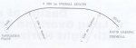
Fig. 1: Plan of conveyor route

The original layout considered elevating the conveyor over the major road and rail crossing. The 7 m elevated gantry would have had to span approximately 100 m. The cost of the steelwork, with the danger of wash-down and spillage onto the road or the rail eventually resulted in the decision being taken to cross the road and rail underground. The crossing itself is also in one of the horizontal curves and this would have made the elevated option more difficult and costly than would normally be the case, given that the gantries would have had concrete floors.

At the two minor roads, the conveyor crossings were both achieved by means of concrete culvert and ramps on each side.

The coal had to be discharged into a 6,000 t holding silo, at 49 m above ground, before being conveyed across another road into the RLT complex. To allow for a second feed to another holding silo in the future, it was decided to stop the overland conveyor short and transfer onto a second conveyor to the silo.

The conveyor therefore has an overall net fall of 13 m from the tail to the head. The lowest point on the conveyor carrying strand occurs at the approach to the head end. This point is at -21 m with respect to the tail.

The drive pulleys are located on the ground behind the head pulley.

3. Design Procedure

3.1 Static Design

Based on the above conveyor requirements, the initial static design was undertaken according to the usual AAC design procedure [1] and produced the following results:

3.2 Dynamic Simulation

The use of static design techniques alone is adequate in the case of short plant conveyors where belt flexibility does not significantly affect the behavior of the belt during starting and stopping. However, in the case of long overland conveyors, where tension waves generated at drive and braking pulleys take a considerable amount of time to propagate along the length of the flexible belt, more detailed dynamic analysis is required to ensure acceptable system behavior under start-up and shut-down conditions. Elements of system behavior that cannot be adequately predicted using static analysis alone include peak belt tensions, displacement of gravity take-ups, belt slippage over drive pulleys and forces generated in holdback devices.

Dynamic analysis of the overland conveyor was carried out within AAC on a 386-PC using ACSL (Advanced Continuous Simulation Language). This is a general purpose language, based on FORTRAN, designed to help the engineer to mathematically model and analyze the behavior of continuous-time systems. In ACSL, the system to be simulated is defined using linear or nonlinear differential equations. These are then integrated numerically over short time steps to produce time histories of system response. ACSL has been used in the Mechanical Engineering Department since 1989 to model various systems, mostly winder related.

The model of the conveyor consisted three main elements: (1) the mechanical subsystem comprising the belt, idlers, take-up, pulleys, reducer and later the fly-wheels; (2) the drain-type fluid couplings and their associated oil-flow regulating system; and (3) the induction motors.

3.2.1 Mechanical Subsystem

In modeling the belt, only axial motion was considered. Although lateral motion of the belt in the tight horizontal curves was an important design consideration, the strong damping of lateral motion allowed adequate predictions to be made using static equilibrium calculations based on dynamically simulated belt tensions.

The mass of the belt; idlers and load material was represented by 32 lumped masses evenly spaced along each of the carrying and return strands (as shown in Fig. 2). The masses were connected by springs which were linear under tension but exerted no compressive force. Motion of the masses was resisted by Coulomb friction elements with friction constants set to correspond to the composite friction factor used in the AAC static analysis. Since the steel cords dominate the elastic behavior of the belt chosen for the conveyor, the more complex viscoelastic behavior of the rubber which needs to be modeled when using more flexible belt constructions), was ignored. Nonlinear stiffness effects introduced by sagging of the belt between the idlers was also considered to be a secondary effect and was ignored. Due to the high stiffness of the short lengths of belt connecting the head pulley and the two drive-pulleys, these three inertias were treated as a single node with rigid connections. Intermediate tensions and the tension ratios across the drive pulleys were calculated using the principle of dynamic equilibrium.

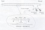
Fig. 2: Conveyor Mechanical Model

The vertical topography of the conveyor was used in the model to calculate, for each belt node, the component of belt and load weight acting axially to the belt.

The number of nodes in the carrying and return strands can be varied. In this way, a sensible balance between accuracy and computation speed can be determined. It was found that, contrary to expectations, as few as 10 elements in each strand are sufficient to predict the primary dynamic effects during start-up and shut-down.

3.2.2 Modeling of Fluid Couplings

The fluid coupling transmits torque generated by the induction motor to the drive pulley via the reducer. The amount of torque transmitted depends primarily on (1) the volume of oil in the coupling and (2) the speed of the output shaft relative to that of the input shaft (referred to as slip).

Characteristic torque-slip curves are supplied by coupling manufacturers. The curves for the Voith 487 TPE coupling (see Fig. 3) were defined in the ACSL model as a matrix of torque values. During a simulation, torque was calculated by two dimensional interpolation using the input and output shaft speeds and the volume of oil in the coupling, all of which were state variables of the system.

The rate Q_out at which oil drains from a Voith 487 TPE coupling when rotating at rated speed can be approximated by the following nonlinear equation supplied by the coupling manufacturer.

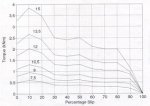
Fig. 3: Characteristic torque-slip curves for fluid coupling (for various oil volumes in litres)

Q_out

= 0.0475 √F(15-0.25f) + 0.317

where: Q_out is in litres/sec
F is the volume of oil in the coupling in litres.

Oil flow into the coupling is controlled by a solenoid valve in an on-off fashion (Q_in is either 1.0 l/s or zero).

The volume of oil F(t) in the coupling at any time was obtained in the ACSL program by integrating the nett flow rate of oil, i.e.

F(t) = ^t∫₀ [Q_in(t) - Q_out (F,t)]dt

3.2.3 modeling of Induction Motor

The induction motors were represented in the ACSL model by the equation of the non-transient torque curve given below (Fig. 4). However, since fluid is only pumped into the couplings once the motors are running in the steep operating region of the curve, motor speed variation has minimal effect on the dynamics of the conveyor. A constant speed representation of the motors would be adequate for most start-up and shut-down simulations.

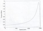
Fig. 4: Characteristic of a 132 kW induction motor

3.3 Changes to Solve Dynamic Problems

Arising from the dynamic analysis, a number of changes were made to aspects of the conveyor configuration to solve problems which arose.

3.3.1 Increased Take-Up Tension

The preliminary selection of take-up tension (14 kN) was inadequate to overcome belt slip on start-up, as evidenced by comparing the tension ratios (T1/T2) across the drive pulleys with the critical value of 3.2 (see Fig. 5). Hence the take-up tension was increased to a minimum of 20 kN.

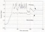
Fig. 5: Tension ratios across drive pulleys

3.3.2 Extended Start-Up Time

The static design calculated the conveyor start-up time to be 38 seconds. On simulating the start-up, high peak tensions were produced. These high tensions were reduced by extending the start-up time to 120 seconds (Fig. 6).

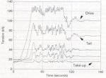
Fig. 6a: Belt tensions (start-up)

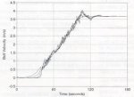
Fig. 6b: Time (seconds)

3.3.3 Control of Maximum Torque During Start-Up

To maintain the start-up torques below the limit of the electric motors, and to achieve the extended start-up time, a maximum start-up torque limit was imposed and used to control the power applied by the motors. This was achieved in practice by controlling the oil flow into the fluid couplings using an on-off solenoid valve. Fig. 7 shows the "saw-tooth" torque profile during acceleration of the belt to full speed. The very long accelerating time, however, required the installation of bigger (160 kW) motors to minimise the thermal effects of the extended accelerating period under full load.

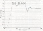
Fig. 7: Primary drive fluid coupling torque

3.3.4 Control of Shut-Down Using Flywheels

On shut-down it was found that theoretically "negative" tensions were developing in the carry strand (Fig. 8). To solve this, the take-up tension was further increased to 30 kN and inertia, in the form of a flywheel, was added to each drive unit. The alternative of a tail brake was rejected as an inferior solution to flywheels. The improved shut-down tension behavior is shown in Fig. 9.

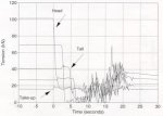
Fig. 8: Belt tensions (shut-down)

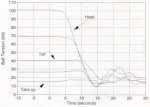
Fig. 9: Belt tensions with flywheels (shut-down)

3.4. Increased Capacity

The future capacity of 1,500 t/h was allowed for in the static design and the dynamic analyses. It was found that the following aspects would have to be changed, as indicated in Table 1.

To allow for these changes, the drive base frames were manufactured for the future condition, with adapters to suit the smaller components. The take-up tower and counterweight were designed for the maximum load (18,000 kg). The flywheel was designed to allow for additional annular rings to be bolted onto the primary disc to increase the inertia. The structure was designed to accommodate the maximum expected tensions.

Table 1: Comparison of parameters for the increased capacity

4. Choice of Drive System

4.1 Fluid coupling

Fluid couplings are well known in mechanical drive systems to accelerate loads with high inertia.

Differential-flow (acceleration control) couplings were chosen for this application due to their simplicity, cost effectiveness, ability to control the belt start-up to any desired format and the facility to run the conveyor at belt inspection speed without the use of a separate pony drive.

Each coupling consists of a normal traction coupling surrounded by an oil-tight enclosure (Fig. 10). The rotor is fitted with orifices in the periphery. The coupling is initially empty of oil. The drive motor is started under no load. Oil is then pumped from a separate reservoir, through a solenoid valve, to the rotor. As the coupling fills with oil, torque is transmitted to the output stator which steadily accelerates. Oil continuously drains from the coupling, but the coupling fill is determined by the higher flow entering the coupling (hence the term "differential-flow").

Fig. 10: Fluid coupling

To limit the torque transmitted and thereby extend the start-up time of the conveyor, the solenoid valve is closed for short periods of time thus momentarily reducing the coupling fill. Control of the solenoid valve is effected by measuring motor power through a PLC.

Fig. 11 shows the layout of each drive unit.

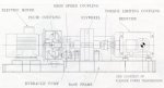
Fig. 11: Drive Unit

4.2 Belt Inspection

By setting a needle valve in the hydraulic circuit the oil fill can be markedly reduced, and the coupling slip increased. This is employed to reduce the belt speed to about 1 m/s for belt inspection purposes. From the elevated slip conditions, the heat gained by the oil is dissipated in an airblast radiator fitted in series in the hydraulic circuit. Thus, separate pony drives are obviated.

4.3 Assessment of Electrical Variable Speed Drive

Early in the project, it was decided to investigate another drive system: an AC variable speed drive. The choice of drive was a pulse width modulated (PWM), current-controlled inverter feeding a squirrel cage motor. The same arrangement of the drive units on the primary and secondary pulleys was used, but each motor would drive the same reducer directly.

AAC, requested the Department of Electrical Engineering of the University of the Witwatersrand (WITS) to collaborate with simulation work. The complete drive system was simulated, including the supply, the converter, the motor and the mechanical load. The conveyor model, developed by AAC, was used as a sub-system of the WITS in-house package.

The work demonstrated that an AC variable speed drive was technically suited to drive the conveyor. However, it was decided to continue with the fluid coupling option on the basis of cost, simplicity, ease of trouble-shooting, and standardization with other drives.

5. Design Audit

A design audit was contracted to Bateman Materials Handling Limited, using the computer software as developed by Conveyor Dynamics Incorporated of the USA. Work progressed, on a co-operative basis with AAC, to refine the mechanical details.

The audit procedure consisted of undertaking a dynamic simulation of the starting and stopping cycles of the conveyor, as statically designed by AAC, under various load conditions.

5.1 Shut-Down Analysis

Shut-down simulations (power outage) confirmed that the conveyor was subject to major tension fluctuations, during stopping, which would adversely affect the ability of the belt to remain in the troughing idlers in the horizontal curves. Braking or inertia devices were suggested. Further simulations were undertaken to optimise the size of the chosen flywheel, with the aim of achieving the smoothest possible shut-down profile on both the velocity and tension distributions. Figs. 12 and 13 show the resultant effect of the flywheel. Also, the flywheel has the effect of reducing take-up movement from a predicted 4 m travel to 1.3 M.

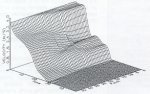
Fig. 12: Velocity profiles on shut-down

Fig. 13: Tension profiles on shut-down

5.2 Start-Up Analysis

The procedure adopted for the start-up analysis followed the same format as the shut-down analysis. Once the relevant performance curves were obtained from the fluid coupling supplier, the torque/time parameters were incorporated into the model which allowed for the simulation of the start-up sequence. This same procedure would apply to any soft-start system.

5.3 Aborted Start Analysis

To conclude the analysis, a series of "what-if" scenarios were undertaken, revolving around the aborted start, i.e. the tripping of the drive motors when belt tensions were peaking during start-up.

This work concluded that, even under extreme conditions, tension waves could not be generated which would adversely affect the performance of the conveyor in the horizontal curves. This was as a result of the damping effect of the flywheels.

5.4 Idler Banking in Horizontal Curves

Having obtained full tension profiles, at points along the length of the conveyor, from the starting and stopping cycles of the conveyor, it was then possible to analyse the curve geometry and calculate idler banking angles. The horizontal drift of the belt was determined, using a gravity principle, throughout the tension profiles, for various idler banking angles.

Thus, by being able to predict the tensions at the horizontal curve tangent points, it was possible to calculate the expected belt drift for various load conditions. Table 2 shows a typical simulation output.

Table 2: Expected belt drift in horizontal curves

From the above it can be seen that the expected belt displacement about its centreline will vary between 75 mm inside the curve to 40 mm outside on the carry strand and between 25 and 50 mm inside on the return strand.

5.5 Idler Rolling Resistance

The idler rolling resistance was considered to be critical for the successful operation of the system, and continues to be so. There have been cases in the past, where long overland conveyors have required every other carrying idler set to be removed during commissioning, in order to get the belt to start initially. This process had to be repeated with alternating idler sets until they had been run in. The cost and duration of such commissioning was completely unacceptable, and the idler manufacturer was required to provide proof of the idler roll breakaway force. Values of a random sample of idler rolls, both carry and return, were taken. The idler rolls were tested on a continuous basis, in order to guarantee the results. A breakaway force of not more than 1.5 N was required.

The results of an analysis of a sample batch are shown in Table 3.

Table 3: Analysis of sample batch

The spread of the breakaway force of the idler rolls tested is illustrated by the histogram in Fig. 14.

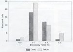
Fig. 14: Idler roll breakaway force

The average values for the breakaway force were 1.20 N for the return idler rolls and 1.18 N for the carry idler rolls, both well within the limit of 1.5 N specified in the dynamic analysis. Attention is being given to quantifying this aspect in the form of running resistance values in a revision of the national standard, SABS 1313 [2], currently under review.

6. Construction and Commissioning

6.1 Overland Structure

In order to reduce capital expenditure, a source of used conveyor structure was found and the sections designed into the overland portion of the conveyor. The structure was designed for a 1,050 m wide conveyor and was equipped with a dog-house on open stringers without deckplates. The sections are in 3.0 m lengths, with angle legs.

The use of second-hand structure required considerable preparation of the steelwork, though, and all the steel was sand-blasted and painted on site. The elevated portions of the conveyor, at the tail and at the head, were equipped with new steelwork, purpose-designed to cater for the belt turnover and the elevation into the drive and transfer house. The overland conveyor stringer modules were supported in augured holes filled with concrete after alignment for most of the overland section of the conveyor. Elsewhere, the structure was supported on concrete sleepers where the ground was undermined.

6.2 Tail Curve

A critical area was the tail curve, where the conveyor profile dipped under the road and rail crossings. The tunnel was constructed in straight sections, each approximately 100 m long.

The construction was a simple rectangular culvert-type tunnel, with the soffit not quite 2.0 m above the finished floor level. The conveyor steelwork was designed to be hung from the soffit, with the vertical hangers welded to cast-in plates after alignment. The initial conveyor installation followed the wall, thus there was no horizontal curve in that area, only three straight sections.

The belt did not bed down properly in the curve and a good deal of lateral drift was experienced at first start-up, particularly in the tunnel area. The belt horizontal line consisted of a series of interlinking curves of varying radius, some as low as 350 m, (the reason for the belt climb-out in the tunnel). In addition, the design vertical curve into the tunnel was not followed, with the result that the belt actually lifted out of the idlers in that area, with the accompanying uncontrolled drift to the inner curve.

A survey was carried out in order to establish the correct conveyor set-out line in the tunnel. When the structure was corrected, the belt performed well. The return idlers were spaced at 6.0 m in the tunnel, instead of the design requirement of 3.0 m. The result was that lateral drift was experienced in certain areas in the tunnel, with the belt drifting heavily into the structure on the inner curve. The return idlers were banked in these areas, up to about 100 and more. However, additional idlers were installed and the banking angle reduced to 4.

6.3 Idler Banking

The idlers on both the carrying strand and return strand were adjusted along the full length of both horizontal curves, in order to achieve the best lateral location of the belt under the varying conditions. In a number of places in the curves, 'punches" were installed, over a distance of about 5 idler pitches, on the carrying strand only. The punch was a set of idlers where the banking was much higher than normal. This has the effect of punching the belt back into line, should excessive drift occur. The normal banking angles in the curves were 60 at the head end carrying strand, 40 at the tail carrying strand and 2 for both the head and tail return strand curves. There were places where the banking angle was increased by packing, to cater for inaccuracies in erection and construction. There was a lead-in to each horizontal curve, over 10 idler pitches, where the conventional carrying idlers were banked in steps to smooth the belt approach and depart sections in the curve. After successful commissioning, the punches were removed and the belt allowed to settle down normally.

7. Testing

After the completion of commissioning, tests were carried out to compare actual performance to predicted performance. The test method was as follows.

7.1 Test Method

The conveyor was run through the cyclic phases of start-up, steady state and shut-down whilst being loaded to 0% (empty), 70%, 100% (rated capacity) and 120% (20% overload).

During the steady state periods, manual readings were taken of:

        motor speed (rev/min)

        fluid coupling output speed (rev/min)

        motor voltage across each pair of phases

        motor current for each phase.

The time to start and stop was taken with a stopwatch, whilst monitoring the fluid coupling output speed with a non-contact tachometer.

During the transient start-up and shut-down periods, recordings were made of the following parameters:

        motor power (kW) for each motor

        belt speed (m/s) at the head and drive pulleys

        take-up displacement (m).

7.2 Results

Fig. 15 shows a typical motor power trace whilst starting a loaded belt. The initial gradual increase of power delivered reaches a maximum when the upper power limit cuts the oil flow to the coupling and the coupling fill diminishes. The lower power limit signals the oil to fill the coupling again. The resultant saw-tooth profile continues until the entire belt is up to speed and the absorbed power drops to normal operating levels.

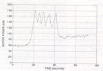
Fig. 15: Motor power (start-up)

All three drive units shared the power requirement equally; typical steady state values were 92, 97 and 94 kW at 1 00% load. Manual reading confirmed the transducer readings. There was an average 3% slip over the fluid couplings at rated belt capacity (100% load).

7.3 Comparison with Design

The graphs (Figs. 16, 17 and 18) show the predicted plots for the loaded start showing anticipated power draw, belt velocity at the drive pulley and take-up displacement, respectively. Superimposed on these curves are the actual measured values.

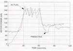
Fig. 16: Comparison of motor power (start-up)

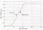
Fig. 17: Comparison of velocity (start-up)

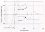
Fig. 18: Comparison of take-up displacement (start-up)

It can be seen that both the motor power and belt velocity curves compare favorably. The predicted curves wore obtained by re-running the simulation after lowering the friction factor from 0.022 to 0.017. This is consistent with the idler rolling resistance as discussed in section 5.5. Having tested the rolls, it was discovered that the breakaway force was generally 1.0 - 1.2 N, which is over 20% lower than the design factor of 1.5 N, resulting in a power saving of approximately 10%.

With regards to take-up displacement, as indicated in Fig. 18, a reasonable correlation can be seen between the predicted and actual readings with regards to the expected travel path. However, the theoretical analysis overstated the magnitude of travel, probably because of the conservative estimation of belt modulus. The start-up and shut-down times for a loaded belt were 65 s and 44 s respectively. Although the start-up time is less than the anticipated figure of 120 s, no dynamic problems have been experienced. The lower start-up time was probably due to the reduced idler rolling resistance coupled with the high power control levels selected in the PLC.

8. Award

The conveyor has been running successfully since being commissioned in October 1992. In the first 7 months of operation, 500,000 t of coal were conveyed to the RLT. This realised the intentions of the project planners in transporting coal from the new Navigation Plant to the export terminal.

The conveyor system was recognised in August 1993 by receiving a 1993 Projects and Systems Award from the South African Institution of Mechanical Engineers.

9. Conclusions

As part of the development of the new Landau Colliery, a 3.2 km overland conveyor, with tight horizontal curves, was designed, commissioned and is running successfully.

The static design and dynamic simulations were carried out within the Anglo American Corporation of South Africa Limited. Arising from the dynamic analysis, a number of changes were made to aspects of the conveyor configuration to solve problems which arose.

Although a variable speed electrical drive was shown to be technically suited to the conveyor, a fluid coupling was selected to control the belt start-up. Additional inertia, in the form of drive flywheels, was added to extend and control the belt shut-down.

Acknowledgements

The authors wish to thank the Anglo American Corporation of South Africa Limited, and the Anglo American Coal Corporation (Amcoal), for permission to publish this paper. The support of Mr. G.O. PARNELL, Consulting Engineer of Amcoal, for this work is recognised.

The assistance of staff in both the AAC Mechanical Engineering and Electrical Engineering Departments is gratefully acknowledged. Members of the WITS Department of Electrical Engineering contributed to the assessment of the electrical variable speed drive. Bateman Materials Handling Limited assisted in the auditing and commissioning of the conveyor. The staff of the Navigation Plant and the Rapid Loading Terminal cooperated with commissioning and field testing. Surtees & Son (Pty) Ltd assisted in carrying out some of the test runs with their measuring equipment.

The committee of the International Materials Handling Conference - Beltcon 7, has given permission for this paper to be published in bulk solids handling.

References

1.      PAGE, J.L. and SHORTT, G.G.: Belt Conveyor Design Criteria within the Anglo American Corporation; international Materials Handling Conference - Beltcon 6, 1991.

2.      SABS 1313: The Dimensions and Construction of Conveyor Belt Idlers and Rolls.

Appendix

Final Specification of Conveyor: