INTRODUCTION TO THE RIDDLE
A RIDDLE OF FRICTION
BY LEONARD S BARNISH
M.C., Pr Eng., C Eng., MA (Cantab) FIMH. MIMechE. MSAIMechE.
Published by:
L S Barnish & PartnersTo
Bridget, without whose cherishing
this would not have happened.
No man can reveal to you aught but that which already lies half asleep
in the dawning of your knowledge.
Kahlil Gibran 1923
Copyright L S Barnish 1993
PART OF THE SERIES A WAY FORWARD
ACKNOWLEDGEMENTS
I am eternally grateful to the late Jim Brear of Clare and Denstone. He provided my first glimpse of communicating with figures.
I am indebted to the Sutcliffe family and Tony Jackson of Robins Conveyors and Hewitt-Robins, for 24 years of experience combined with fun.
My thanks go to all two hundred clients who supported my practice with their problems.
Lastly, but by no means least, Rudi Urmann, friend and associate, the only engineer Ive known with professional "greenfingers".
A few short hours before printing this slim volume, Michael Sara, FRCS, provided me with some post knee prothesis convalescent reading. This included Messrs Streicher, Schon and Semlitschs paper entitled "Investigations of the Tribological Behaviour of Metal-on-Metal Combinations for Artificial Hip Joints". The similarity of principles with what follows herein are intriguing.
INTRODUCTION TO THE RIDDLE
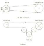
During the last two hundred years of the Industrial Revolution, literally billions of mechanical power transmission systems have been built using an Endless Belt and Pulleys (Figure 1).
These mechanisms are still very successful and have progressed to individual units handling up to 4 Megawatts. All of this despite there being no precise explanation as to how the friction between Belt and Pulley actually works.
I was introduced to this quite extraordinary situation in the form of an unsolved Riddle, "What are the mechanical principles of friction where there is relative movement at the interface". Desmond Sutcliffe, grandson of Britains pioneer in Belt Conveying in Coal Mines, gave it as a priority item in his research and development briefing in the summer of 1948.
What follows is an interpretation of some of the past research and what can be observed from simple experimentation.
SOME OF THE PERTINENT FACTS
The belts used in the early mechanisms were tanned leather; taken from the animals back for the "best quality" and used with the hairy side, though shaved, to achieve premium friction values on the contact face of the Drive Pulley. Today the constructions include tensile reinforcement of natural and synthetic fabrics in woven plies, or steel cords, all enclosed in a matrex of Rubber or P.V.C. The common factor is that they are elastic with varying moduli, and known as Elastomers.
When power is transferred between a pulley and an elastomeric belt there is a difference in belt tension or Stress between the "on coming" and the "off-going" portions. The elastic Modulus or Stress/Strain quantifies the amount of contraction or elongation strain. Therefore there has to be a physical movement between the belt and the pulley face.
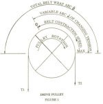
In operation, around a Drive Pulley, belts contact the pulley in a stretched state and contract in length over an arc (α), which always starts from where they leave the pulley, but which may vary from zero, when no power is applied, to a maximum coinciding with the initial contact point. The contraction always takes place in the opposite direction to the drive pulley rotation but in the same direction when the belt drives a pulley (Figure 2).
Researchers using stroboscopes, prior to the second world war, identified varying speeds of belt contraction on a Drive Pulley. They noted that the highest speed occurred just before the belt left the Drive Pulley, which coincides with the lowest point of tension (Figure 2). They knew, from research at the turn of the century, that the ratio of high to low tensions T1/T2 = eα where was only the mean coefficient of friction. Despite also knowing from this, that if α exceeded the total wrap, θ, of the belt around the pulley, or when T1 - T2 = Te was excessive the belt would start to slip totally on the pulley surface, but inexplicably up to an undetermined point it would transmit an overload before uncontrollably skidding.
Most belt power transmission designs today still use the empirical formula based upon T1/T2 = eθ. The θX representing the total wrap of the belt around a drive pulley and the varying mean coefficient of friction, normally from 0.25 to 0.35 for different contact faces plain steel or cast iron to lagged with rubber, even though they know the mean coefficient is at least two hundred and fifty per cent greater (Figure 3).
Since there was no explanation of interface friction increasing with the higher contraction or creep speeds and many other characteristics, the belt manufacturers and the rubber technologists concede their knowledge of the matrex component of the belts as limited. Therefore the construction was and still is, in fact, an ART FORM where development becomes dependent upon laboratory comparative testing but not precisely predictable.
The first glimmer of change occurred, after the second world war, as the use of rubber became even more popular in industry for such things as: -
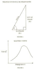
Bicycle and Motor Car tyres, Vibration, Shock absorption and flexible Bridge Mountings. Researchers produced a Master Curve for identifying many combinations of elastomers characteristics made from different polymers or mixtures. This curve was compiled from a "triangle of Elastic Moduli" occurring at different frequencies or speeds of deformation (Figure 4). The "components" were the Moduli Vectors when subjected to "in line" or "in phase" E1 deformation (this was the base of the triangle). The second being the "Out of Phase" E2 occurring at right angles to the base, and the hypotenuse was the "Total". The angle between the base and hypotenuse was referred to as X and tan X plotted against the frequency made up the Master curve. The form is similar to that for the Law of Probability.
These same Researchers noted without much emphasis that "strain rate" could replace the Modulus component.
The major characteristics are that it predicts a Peak at a particular frequency. Also if the operating temperature increases the peak moves eastward and when it decreases it moves westwards as coincides with hardness of the rubber (Figure 5). Other facets are that not only different polymer mixes but cooking or curing of them are displayed.
The creation of this Master Curve is unquestionably complex but not quite as bad as Crick and Watsons D.N.A. But it does provide collaborating evidence that an elastomers speed of deformation or creep in a belt has a quantifiable peak as observed in the early nineteen hundreds but which remained unexplained for 50 years.
The exponential increase in tyred vehicles in the 1950s and 1960s provided the boost for further research in order to provide safer road holding or frictional grip. This prompted the Rubber Industry and particularly those involved with car racing to re-assess the Leonardo Da Vinci and Coulomb laws of friction.
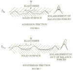
By the 1970/80s men like Desmond Moore had clearly established that there were two distinct types of elastomeric or visco elastic frictional forces, both dependent upon the magnitude of the force normal to the interface (W). The first being an "Adhesive" shear coefficient acting at the contact faces but depending upon area, (Figure 6). This latter is critical since a surface such as a road may have rounded or pinnacle asperities upon which the rubber will drape itself so that the actual area can be less or even more than, say two perfectly smooth surfaces.
The second type is "Hysteresis" related and involves relative movement at the interface when the elastomer drape formation is not uniform each side of the asperity (Figure 7).
The initial elastomer contact with the asperity is lower than that when it leaves that same asperity. The effect is frequently called "bulking". The phenomena is affected by the depth of distortion and its natural desire to revert increases the magnitude of this particular friction. This behaviour therefore involves more than just the immediate contact surface.
Further experimentation under varying creep speeds including wet, dry and icy conditions produced a basic mathematical model covering both Adhesion and Hysteresis.
Showing the frictional forces: -
FT = FA + FH
The Coefficients of friction and the normal force (W) are: -
WT = WA + WH
and T = A + H
Where 1)
A = K1 x S (Shear Strength N/mm2) x tan δ x E1 (In Phase Modulus) / P
Where P the pressure = W / The Actual Area
and 2)
H = K2 x P x tan δ / E1
Again where P = W / The Actual Area
and 3) the constants are related by :- K2 = K1x K3
During the development of the adhesion formulae they noted that the actual relative movement of the elastomer over the asperities was not a perfectly smooth action. The movement they referred to as Stick/Slip denoting that the Stick period comprised contracting and bonding between the contact surfaces and the slip being the rupturing and relaxing, before new bonds were formed.
For years the Belt Conveyor Industry has been criticised for the lack of product development. One such reproach likens the current conveyor designs to an early model car lying upturned on its roof with the road running over the wheels. This is a reasonable analogy when you consider todays sophisticated suspension systems.
However, the idea of using an analogy to initiate change is an attractive one and so the critical association with cars seems apt. Consider the draping of a motor cars tyre over an asperity in the road as analogical to a belt wrapped around a drive pulley.
A simple set of tests appears to confirm the relationship.
EXPERIMENTAL COMPARISON
Since it has always been difficult to see the creep or relative belt movement on a rotating driving pulley, stop the pulley and leave it so.
1) Then attach a sample of the Elastomer to the surface of a pulley and allow it to hang freely under a predetermined mass, equating to a truly representative stress in the sample. Measure the reducing strain against the change in stress by eliminating the mass little by little. Beware that an unworked rubber will give wild results! Also remember your own skin is an elastomer and needs movement to reduce ageing - so too does rubber! In order to eliminate some of the incompressible characteristics of an elastomer record the strain as
(λ - λ-2) where λ is the ratio of [original lengths] / [final lengths], i.e. the results are all > 1.
These results are in fact the In Phase type of Strain or Strain1
Calculate the mean contraction speed based upon the simple harmonic theory: -
Plotting the Strains (λ - λ-2) against V / 2 provides "In-phase" Strain1 Rates.
2) Now reload the elastomer to the same reasonable maximum stress (Figure 8).
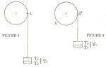
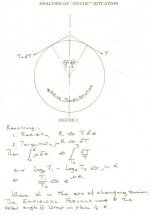
Then very slowly wind up the belt around the pulley to say +- 230 degrees. Now the whole sample is at a uniform tension of Ti. But remember that the bending strain in the belt has reduced the stress at the contact face (Figure 9).
Mark off the Pulley surface and the bottom edge of the elastomer in 5deg or 10deg (depending on the size of the sample and the pulley) increments, including some equivalents on the free hanging length.
NOTE: always take measurements well clear of the fixing points on the pulley and where the masses are attached.
3) Now slowly remove the mass representing Te leaving that for T2 still attached. Note that the Point 0deg on the Belt moves rapidly and then decelerates to a static point as the internal Restoration Force Wave passes.
Record the new static locations of the beltmarks to those on the pulley surface.
Calculate (λ - λ-2) for each marked point and on the basis that each segment of the belt has accelerated from rest to a maximum speed, under the influence of the Restoration Force in the elastomer, and then decelerated back to zero speed. All this occurs to each point that is displaced. Using the change in angular momentum as a basis for the mean speed attained during the acceleration determine
Now plot λ - λ-2 against V / 2 which provides the "Total Strain T" Rates
Note carefully that the bending stress should be used for adjusting the Total T2at the 0deg point since the bending strain takes place over an arc -13 to +13.
Since the primary interest is of Adhesive conditions, reduce all strains to λ - λ-2 / Cross Section of Sample mm2
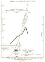
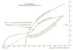
4) Now plot the findings from paragraphs 1) and 2) as illustrated in Figure 10. The triangle of changing Strain Rates (In-phase and Total) can then be formed for various mean speeds, from which the angle X can be determined. This enables the Master Curve to be plotted as tan X versus the mean speeds.
4.1. Remember: - A Master Curve for a Rubber compound with a higher Elastic Modulus or High Hardness will have a peak tan X occurring at a much lower mean speed.
The characteristic of the elastomer hardening with increased strain rate is common to all visco elastomers.
But where tensile reinforcements are included in a belt the interface will normally be subject to a lower strain rate albeit with a higher normal loading (W).
4.2. In the Adhesion Formula A = K1 x S/P x Strain1 Rate x tan δ
Since the product Strain1 Rate x tan δ, at a constant Operating Temperature and on a given surface, is proportional to speed, then the coefficient of friction A will have a similar shape as the Master Curve.
4.3. The reverse curve at the beginning of the Master Curve occurs due to the rapid rate of change occurring between the TOTAL StrainT Rate in relation to IN PHASE Strain1 Rate.
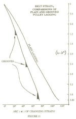
5) By repeating these steps with the surface of the pulley grooved the variation in angle of changing StrainT is obvious (Figure 11). Hence provided the elastomers bending characteristic is capable of being deflected into the groove there will bean Hysterisis effect. From that it is clear that the total friction coefficient T is greatly increased.
5.1 It is perfectly possible to generate and vary Hysteresis components
a) from a smooth undulating surface as illustrated on page 12, Figures 6 or 7
and
b) from changing bending strains.
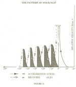
6) Figure 12 illustrates that the pattern of relative movement (or creep) is related to Power Transmission.
6.1 The pattern has been developed from observations of 10 segments.
6.2 the shaded portion is one of Acceleration from zero relative velocity to a maximum and then back to zero. Rubber Technologists refer to this as STICK/SLIP. In fact the Acceleration segments represent TRANSMISSION OF POWER whereas the "dotted outline" is the RELAXATION against a reduced frictional resistance force, after the Restoration Wave Force has passed onto the next segment.
SUMMARY
A reconciliation of the experimental findings with Moores Tyre Formulae confirms:
a) That a smooth rounded dry surface has only a small component of Hysteresis type of friction and the majority is of an Adhesion type.
b) Grooving of one surface may well increase wear, but a wavy moulding matching the bending and other characteristics of the second member would have just as good a Hysteresis result. This can occur especially with a booster type belt with higher loads over supporting idlers or pressure pulleys on Drive Pulleys, and relative speeds resulting from one belt contracting and the other stretching in unison.
c) The reverse curve on "tan δ" at the low speed end originates from high rates of change of Module or Strain this area. (Figure 10 on page 18). This same characteristic was detected in analysis of the N.C.B. experiments, in 1956. But the effect is overshadowed with Hysteresis in a grooved surface.
d) The Master Curve "peak" triggers the change in the arc (α) when V/2 exceeds the Peak speed. Then since its friction coefficient declines a greater arc evolves.
WHAT NOW?
With a simple means of experimenting and a neat means of quantifying the results there is now surely less excuse for accepting any past analogical criticisms of Belt Mechanisms. But it becomes a possibility to use these additional characteristics as a basis for improved methods and products.
A little further away is the potential to not only "Increase" but also "Reduce" friction now that there is hopefully better understanding of interfaces including such examples as:
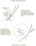
A "Drop Shot at Tennis on different court surfaces",
A "Golfers inability to stop his chip shot from the rough onto a hard surface."
It is pertinent that the belts, years ago, came from our relatives "backs". A future possibility may now exist for components in prostheses from our own backs.
There is little that is new around, we are just a bit unaware. "The elastomeric phenomena discussed here have in fact been an intimate part of our procreation system for the past 40 million years
| 1. O Evans | American, who published a "Millers Guide" in 1795, describing a very early belt conveyor. |
| 2. P Westmacott & G Lyster | UK Engineers at Liverpool Docks, in 1865 experimented with wooden idler rolls. |
| 3. Richard Sutcliffe | UK pioneer mining engineer provided the first underground colliery conveyors. |
| 4. Wilfred Lewis & Carl Barth | 1908/9 presented a paper to the ASME on transmission belts. |
| 5. R G Jones | Professor of Ohio State University, in a paper to the ASME in 1926 described measuring of creep speeds with a stroboscope. |
| 6. H W Swift | In 1927 presented a paper to the Institution of Mechanical Engineers, London, entitled "Power Transmission by Belts". |
| 7. Desmond Sutcliffe | Grandson of R Sutcliffe, instigator of investigation into friction on drive pulleys. |
| 8. Don Clark | ex Leeds University, Messrs. Richard Sutcliffe Ltd. and N.C.B. Scientific Department. Experiments into Stress and Strains imposed on Multiply Conveyor Belting by Flexing 1956. |
| 9. Payne & Scott | Engineering Design with Rubber 1960. |
| 10. Desmond Moore | author of "The Friction of Pneumatic Tyres" 1975. |
| 11. Leonard S Barnish | "The Transmission of Power to high speed Belts". 1989. |
| 12. A Harrison & A W Roberts | "Mechanisms of Force Transfer on Conveyor Belt Drive Drums", 1992. |
![]()