|
On the Application of
Beam Elements in Finite
Element Models of Belt Conveyors |
|
G. Lodewijks, USA
Summary
Beam elements can be applied in finite element models of long belt conveyor systems in order to simulate the belts global elastic response, in both longitudinal and transverse directions, during starting and stopping. The advantage of applying beam elements instead of truss elements is that the coupling between the longitudinal and transverse response of the belt can be taken into account. Comparing the discretisation of a belt conveyor to a finite element model built of truss and of beam elements shows that especially the way the boundary conditions are treated is different. If a mixed model, built of both truss and beam elements, is applied then the simulations will be accurate and not too time consuming.
Nomenclature
| A | cross-sectional area of the belt [m²] |
| D | vector of first order transfer function |
| E | YOUNG'S modulus [N/m²] |
| F | drive force [N] |
| L | total length of the belt [m] |
| Mred | reduced mass of the drive and take-up pulley [kg] |
| MT | weight of the take-up mass [kg] |
| M | mass matrix |
| R | transformation matrix |
| S | stiffness matrix |
| T | belt tension [N] |
| W | mass of a half belt span between two idlers [kg] |
| ei | unit vector in i-direction |
| f | resistance force [N] |
| l | length of a belt span between two Idlers [m] |
| ls | length of belt part between take up and drive pulley [m] |
| lo | undeformed length of belt span between two idlers [m] |
| lij | vector which connects nodal point i with nodal point j |
| q | distributed mass of belt and bulk material (kg/m1] |
| r | radius vector |
| ui | longitudinal displacement of nodal point i [m] |
| vb | average belt speed [m/s] |
| vi | transverse displacement of nodal point i [m] |
| xi | x coordinate of nodal point i [m] |
| x | position vector with reference to fixed reference frame |
| yi | Y coordinate of nodal point i [m] |
| δ | belt sag [m] |
| ε | vector of generalised deformation parameters |
| εs | strain component due to the static geometrical belt sag |
| ξ | relative length coordinate |
| ρ | density of belt and bulk material [kg/m³] |
| σ | vector of generalised stresses |
| φ | angle between the tangent to the belt and the horizontal. |
1. Introduction
Since powerful computer systems are available, finite element models (FEM) and techniques are applied in all branches of engineering. In the field of belt conveyors FEM-techniques are used in two specific applications. In one application they are used to model the conveyor belt in order to determine its global dynamic response during starting and stopping, [11] and [15]. In the other, they are used to model the belt splice in order to determine the local stress distribution and the corresponding breaking strength due to the global response of the belt, [6] and [14]. The first application will be discussed in this paper.
If the total power supply needed to drive a belt conveyor system is calculated with design standards like DIN 22101 then the belt is assumed to be an inextensible body. This implies that the forces exerted on the belt during starting and stopping can be derived from Newtonian rigid body dynamics which yields the belt stress. With this belt stress the maximum extension of the belt can be calculated. This way of determining the elastic response of the belt is called the quasi-static (design) approach. For small belt conveyor systems this leads to an acceptable design and acceptable operational behaviour of the belt. For long belt conveyor systems, however, this may lead to a poor design, high maintenance costs, shod conveyor component life and well-known operational problems like:
-
excessive large displacement of the weight of the gravity take-up device
-
premature collapse of the belt, mostly due to the failure of the splices
-
destruction of the pulleys and major damage of the idlers
-
lifting of the belt off the idlers which can result in spillage of bulk material
-
damage and malfunctioning of (hydrokinetic) drive systems.
Starting with the traveling elasto-mechanic wave model in the early seventies, [4], many researchers developed models in which the elastic response of the belt is taken into account in order to determine the phenomena responsible for these problems. The resistances and tomes exerted on the belt vary from place to place. The belt-model therefore consists of finite elements in order to account for these variations. The global elastic response of the belt is made up by the elastic response of all its elements. The FE models are applied in computer software which can be used in the design stage of (long) belt conveyor systems in order to determine the elastic response of the belt due to starting and stopping procedures. This is called the dynamic (design) approach. Verification has shown that computer programs based on these FE models are quite successful in predicting the elastic response of the belt during starting and stopping, [5] and [15]. The FE models as mentioned above determine only the longitudinal elastic response of the belt. Therefore they fail in the accurate determination of:
-
the motion of the belt over the idlers and the pulleys
-
the lifting of the belt off the idlers
-
the dynamic drive phenomena
-
the bending resistance of the belt
-
the behaviour of the belt in convex and concave curves
-
the influence of the belt sag on the propagation of stress waves
-
the development of shock waves
-
the development of standing transverse waves.
The transverse elastic response of the belt is often the cause of breakdowns in long belt conveyor systems and should therefore be taken into account. The transverse response of a belt can be determined with special models as proposed in [7] and [13], but it is more convenient if existing FE models can be extended with special elements which take this response into account.
In this paper an example of a FE model will be given which can be used to simulate the longitudinal elastic response of the belt. Further, a detailed explanation is given why it is necessary to analyse transverse motions of the belt, and a FE model which accounts for both the longitudinal and the transverse elastic response of the belt will be proposed. Finally, a brief discussion of the question when to apply which model will be presented. The results of simulations with a combined model will be given in Part II of this paper.
2. Modelling the Longitudinal Elastic Belt Response
Before it can be pointed out what the differences are between a FE model used to simulate the transverse elastic belt response and a FE model used to simulate the longitudinal elastic belt response, it should be explained how a longitudinal FE model can be developed.
2.1 Discretisation of a Belt Conveyor
A typical belt conveyor geometry consisting of a drive pulley, a tail pulley, a vertical gravity take-up and a number of idlers, is shown in Fig. 1.
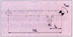
Fig. 1: Typical belt conveyor geometry
The length of the belt part between the take-up pulley and the drive pulley, ls, can be neglected compared to the total length L of a long conveyor system. The take-up and the drive pulley may therefore be combined mathematically in one pulley as long as the mass inertia of the pulleys of the take-up are accounted for. The mass of the take-up system is MT. see Fig. 2. Since the main interest is in the longitudinal elastic response of the belt, the influence of the idlers on the longitudinal dynamic behaviour of the belt can be represented by forces that account for the resistance of the idlers to rotation on their bearings, the resistance of the belt to flexure around The idlers etc. These forces vary from place to place depending on the exact local condition and geometry of the belt conveyor.
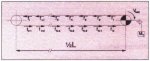
Fig. 2: Take-up pulley and drive pulley combined
The next step is to divide the belt into a number of finite elements. The total forces exerted on a specific part of the belt are allocated to the nodal points of the element which represents that part of the belt, see Fig. 3.
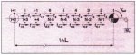
Fig. 3: Belt divided into finite elements
It is not necessary to define elements on those positions in the conveyor where the motion of the belt is enforced by pulleys (no slip possible), for example on the drive pulley. Two forces, F1 and FN In Fig. 4, account for the coupling between the two nodal points which are located on that pulley, the nodal points 1 and N in Fig. 3. The belt is discretised on those places where it is supported by a pulley which does not force its motion (slip possible), for example the tail pulley of Fig. 1. Forces allocated to the nodal points of the element around that pulley account for the resistances in the bearings of the pulley and its mass inertia, see fi+l and fi+2 in Fig. 4. The maximum belt speed is about 10 m/s whereas the speed of the longitudinal stress waves varies from about 1,000 m/s for EP belts to 2,500 m/s for steel-cord belts, Hence, the influence of the belt speed on the elastic response of the belt is negligible. This implies that all the elements and the forces which account for the interaction between the belt and its supporting structure remain in their position relative to the supporting stricture. The bulk material travels through the fixed element grid with the belt speed.
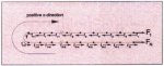
Fig. 4: Replacing the interaction of the belt and its supporting structure by forces
In Fig. 4 the orientation of the elements is given which results in the configuration of Fig. 5 when the belt is laid in the x-direction.
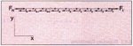
Fig. 5: Belt laid in x-direction
The exact interpretation of the elements depends on which resistances and influences of the interaction between the belt and its supporting stricture are taken into account and the mathematical description of the constitutive behaviour of the belt material. Depending on this interpretation, the elements can be represented by a system of masses, springs and dashpots, see for example Fig. 6, [15], where such a system is given for one element with nodal points c and c + 1.
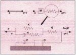
Fig. 6: Five element composite model [15]
2.2 Truss Element
If only the longitudinal deformation of the belt, and not its bending deformations, has to be taken into account then a truss element can be used to model the response of the belt. Some relevant aspects of this element will be discussed in this section.
2.2.1 Deformation Parameters
The truss element shown in Fig. 7 has four degrees of freedom. Each nodal point has two displacement components which define the component vector x:
xT = | up vp uq vq | (1)
Four vectors fix the position of the nodal points with respect the global Cartesian coordinate system:
| rp = xpe1 + ype2 up = upe1 + vpe2 rq = xqe1 + yqe2 uq = uqe1 + vqe2 |
(2) |
The vector which connects the two nodal points of the deformed element is:
lpq = rq + uq - rp - up (3)
In order to describe the position of any point on the element, linear shape function is used. The vector which fixes this position is, in the undeformed state:
rξ = rp + (rq - rp)ξ (4a)
and in the deformed state:
rξ + uξ = rp + up +(rq + uq - rp - up)ξ (4b)
where ξ is a dimensionless coordinate along the axis of the element which varies from 0, in nodal point p, to 1 in nodal point see Fig.7.
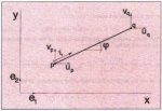
Fig. 7: Definition of the displacements of a truss element
For the in-plane motion of the truss element there are three independent rigid body modes. Therefore, one deformation mode remains which describes the change of length of the axis of the truss element. In order to determine the average change of length of the truss axis, the length of a material line element of the axis is defined. In the undeformed state this length is equal to:
ds²0 = drξ · drξ (5a)
and in the deformed state:
ds² = (drξ + du) · (drξ + du) (5b)
With these lengths the axial deformation of the truss element can be defined by:
| ε1 = D1(x) = | ¹∫o | ds² - ds²o | dξ = | 1 | (lpq · lpq - l²o) + ξo1 (6) |
| 2ds²o | 2l²o |
in which the length of the undeformed element lo, is equal to:
![]()
The function D1 is called a first order transfer function. In Eq. (6) the quadratic length of the material line element is used which is in agreement with the continuum definition of the strain component. The term ξo1 indicates a possible pre-strain. Depending on the belt type the belt material can be taker as linear elastic or linear visco-elastic, [16], also see section 4. If it is to be expected that there are belt sections in the conveyor where (∂v/∂x)² is of the order (∂u/∂x) then it is necessary to take the influence of the belt sag on ε1 Into account. This situation can for example occur in long belt conveyor systems with up-Nil and down-hill sections or after an emergency breakdown, [3].
Although bending deformations are not included in the truss element, it is possible to take the static influence of small values of the belt sag into account. In DIN 22101 the belt sag δ is determined from the equilibrium equations of a tensioned sting which is simply supported at both sides. By definition this is:
δ = ql²/8T (8)
where q is the distributed mass of the belt and bulk material, l the length of the belt span between two idlers and T the belt tension, see Fig. 8. The angle between the horizontal and the tangent to the belt is:
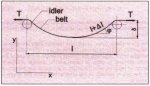
Fig. 8: Static sag of tensioned belt
| φ (x, T, q) = | ∂v | = - | qx | + | ql | (9) |
| ∂x | T | 2T |
where v is the transverse displacement of the belt. Written in terms of the mass of a half belt span, W = (ql)/2. the belt tension T and the coordinate ξ, Eq. (9) becomes:
| φ (ξ, W, T) = - | 2W | ξ + | W |
(10) |
| T | T |
The effect of the belt sag on the axial strain is determined by:
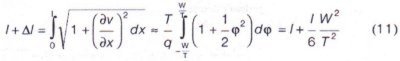
This yields:
|
εs = |
Δl |
= |
l W² |
(12) |
| l | 6 T² |
and the total longitudinal strain:
ε*s = ε1 + εs (13)
2.2.2 Boundary Conditions
As explained in section 2.1 the interaction between the belt and its supporting structure is expressed in terms of forces. These forces depend on the belt speed, the mass inertia of the belt, idlers and pulleys and on the angular velocity of idlers or pulleys. The forces F1 and FN can be determined from their contribution to the equations of motion which can be derived with the principle of virtual power, see section 4:
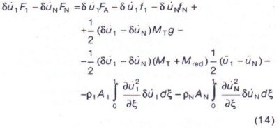
This yields the forces F1 and FN:
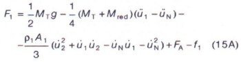
and
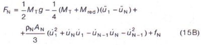
where FA is the drive force. In these equations the only coupling between nodal point 1 and N is through the motion of the take-up mass.
Different kinds of couplings and drives, however, result in different forms of the Eqs. (14) and (15). The forces f1 and fN depend on the running resistances of the belt and can be divided in four groups: main resistances, secondary resistances, special resistances and lifting resistances, see for example [12].
3. Modelling the Total Elastic Belt Response
In Section 2 it was explained how a belt conveyor geometry can be discretised to a finite element model in order to determine the longitudinal response of the belt. It was also shown that the boundary and support conditions can be replaced by adding average (resistance) forces to the nodal points of the relevant truss elements. With this FE model the longitudinal response of the belt can be simulated during the design stage of a long conveyor system in order to prevent problems as mentioned in the introduction, However, a lot of unsolved problems still remain. Most of them are caused by the influence of the belt sag and transverse vibrations on the total response. Although the influence of the belt sag can be taken into account as is shown in Section 2.2, this does not account for the coupling between the transverse and longitudinal displacements and deformations. If the transverse displacements and bending deformations of the belt are taken into account then the belt has to be discretised on such a scale that the motion of the belt between two idlers can be determined. This implies that also the motion of the belt over pulleys, idlers and plates has to be modelled. This is quite different from the longitudinal case where only the interaction between the belt and the pulleys etc. had to be described. Applying such a model in a simulation program enables the determination of the following phenomena:
- the interaction between the belt sag and the propagation of longitudinal stress waves. An increase of the belt sag due to a decrease of the belt tension slows down the propagation of stress waves. If the average stress level of the stress wave is high related to the stress level in front of the wave then the propagation speed of the wave front is lower than the propagation speed of rest of the wave which results In a steep gradient of the stress rate.
- the interaction between an idler and the belt. This interaction is especially influenced by:
- the indentation rolling resistance
- the flexural resistance of the belt
- creeping break-away friction.
- the influence of the belt speed on the stability of the motion of the belt.
- the dynamic stresses in the belt during a passage of the belt over a (driven) pulley.the influence of parametric resonance of the belt due to the interaction between vibrations of the take-up mass and the transverse displacement of the belt.the development of standing transverse waves.the influence of the damping caused by bulk material and by the deformation of the cross-sectional area of the belt and bulk material during passage of an idlerthe lifting of the belt in convex and concave curves especially during starting and stopping.
3.1 Discretising of a Belt Conveyor
The most significant difference between modelling only the longitudinal motion of the belt and modelling both the longitudinal and transverse motion is that in the first case the elements keep their position compared to the supporting structure whereas they move in the second case. The handling of the boundary conditions in both cases is therefore quite different. For the transverse case it is not sufficient just to allocate forces to the relevant nodal points of the elements which account for the interaction between the belt and a support. The exact position of the element on the support also has to be determined to check whether this position is geometrically possible. This procedure has to be repeated every time step and is different for each type of support. Therefore, three types of supports have to be distinguished, the pulley support, the idler support and the plate support. see Fig. 9.
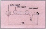
Fig. 9: Three support sections
3.1.1 Idler Support
One specific point of the belt is supported when it moves over an idler, see Fig. 10. The length of the belt between this point and point p can be fixed by a length coordinate ξ. The vectors rp, rid and rq determine the nodal points of the element and the idler with respect to a reference frame.
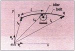
Fig. 10: Belt supported by an idler
In order to enable a mathematical description of the interaction between the idler and the belt two extra deformation parameters. ε4 and ε5, are added to the element which represent the geometrical interaction between the belt and the idler, see Fig. 11.
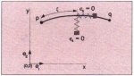
Fig. 11: Idler supported beam element
These deformation parameters can be Imagined as springs of infinite stiffness. This implies that the values Of ε4 and ε5 are zero when the position of the element agrees with the geometrical possibilities. The displacements of nodal point p and q are coupled by forces in order to minimize ε4 and ε5. These forces and also the resultants of the drive forces and the resistance forces are shown in Fig. 12.

Fig. 12: Forces acting on idler supported beam element
3.1.2 Pulley Support
When the belt moves over a pulley it depends on the position of the element whether the whole element or a part of the element is supported. Elements which are supported by the edge of the pulley are partly supported, see Fig. 13. The distance between a nodal point on a pulley and the axis of the pulley is restricted by the radius of that pulley. The angle between the orientation at the nodal point and the horizontal is restricted to the angle between the tangent to the pulley and the horizontal. This is forced by an non-deformable connection rod which is placed between the axis of the pulley and the supported nodal point of the element, see Fig. 14.
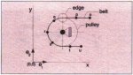
Fig. 13: Belt supported by a pulley
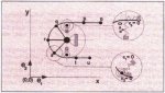
Fig. 14: Pulley supported beam elements
Nodal points of partly supported elements which are not located on the pulley are coupled with the supported nodal point by an idler support which is located on the edge of the pulley. This prevents the edge elements from geometrically impossible displacements. The axis of the pulley is modelled as a hinge element which enables the connection rods to rotate. If belt slip is possible then the angular speed of the connection rods can differ. In this case the plural hinge element shown in A of Fig. 15 can be used, If belt slip is not possible then the angular speed of all the connection rods must be the same and a combined hinge element should be applied when a part of the belt slips over the pulley. The single hinge element shown in B of Fig. 15 can be used.
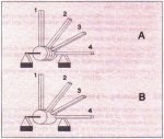
Fig. 15: The axis of the pulley as plural (A) and single (B) hinge element
3.1.3 Plate Support
When the belt moves over a plate then the transverse displacement of the belt is restricted, see Figs. 16 and 17. In order to allow the belt to enter and leave the plate supported section smoothly, two idler supports are used on the edges of the plate.
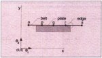
Fig. 16: Belt supported by a plate
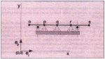
Fig. 17: Plate supported beam elements
3.2 Beam Element
It is sufficient to use truss elements to model the belt if only the longitudinal deformation of the belt is considered. If the bending deformations have to be taken into account then beam elements can be used to model the belt. In this section some relevant aspects of beam elements will be discussed.
3.2.1 Deformation Parameters
Parts of the belt can have considerable transverse displacements and rotations. The local deformations, however, should still be small if only elastic deformations are considered. Therefore, the relative displacements of all material points of a beam element between two nodal points should be small compared to the distance between these nodal points.
The beam element shown in Fig. 18 has six degrees of freedom. Each nodal point has two displacement components and one angle of rotation which define the component vector x:
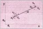
Fig. 18: Definition of the nodal point displacement and rotations of
a beam elementxT = | up vp p uq vq q | (16)
For the in-plane motion of the beam element there also are three independent rigid body modes. Therefore three independent deformation modes remain, The beam element has, besides a longitudinal deformation parameter, two bending deformation parameters which are defined by the projection of the straight line between two nodal points on the unit normal vectors to the centroidal axis of the beam element, see Fig. 19.
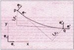
Fig. 19: The bending deformations of a beam element
These bending deformations, ε2 and ε3 can be specified by the inner product of the vector lpq and the vectors εp2 and εq2. [2]:
ε2 = D2 (x) = ep2 · lpq l0 ε3 = D3 (x) = eq2 · lpq (17) l0 The relationship between the local and the global unit vectors is:
eip = R*ij Rpjk ek (18)
where the matrix R* describes the transformation of the global base vectors to the local base vectors of the undeformed state and Rp describes the transformation due to nodal point rotation.
In order to take into account the influence of the bending deformations on the stretching of the centroidal axis of the beam element, the two bending deformations are superimposed on the linearly varying displacements between the two nodal points. In the deformed state the position of any point on the axis of the beam element is fixed by:
rξ + uξ = rp + up + (rq + uq - rp - up)ξ - l0 [ε2ep 2 (ξ³ - 2ξ² + ξ) + ε3eq2 (-ξ³ + ξ²)] (19)
With the Eqs. (4a), (5a&b) and (19) the axial deformation of the beam element can be defined by:
ε1= D1 (x) 1
∫
0ds² - ds²0 dξ = 1 (lpq · lpq - l²0) + 1 2ε²2 + ε2ε3 + 2ε²3) + ε01 (20) 2ds²0 2l0² 30 It is possible that a bended beam has no longitudinal strain in its initial state. Since the bending deformation terms in Eq. (20) will result in an initial strain, it must be possible to correct this. To take this into account the initial strain component ε01 has been introduced.
3.2.2 Boundary Conditions
If the belt moves over an idler then the parameter ξ is added to the component vector x of Eq. (16). Since only two rigid body motions are possible for an in-plane beam element which is supported by an idler, five deformation parameters remain. Three of them determine the deformation of the beam element and are given in Eqs. (17), (18) and (20). The remaining two determine the interaction between the belt and the idler and are shown in Fig. 11.
If the radius vector to the top surface of the idler is given by (also see Fig. 10)
rid = xide1 + yide2 (21)
then the strain component; ε4 can be defined by:
ε4 = D4 (x) = (rξ + uξ) · e1 - rid · e1 = 0 (22)
and C5 can be defined by:
ε5 = D5 (x) = (rξ + uξ) · e2 - rid · e2 = 0 (23)
If, during the simulations, the condition ε4 > 0 occurs then the belt has left the idler and the idler support is removed. The angle φ of the belt can be restricted to the angle φid of the idler or pulley. The deformation parameter ε6 can be used for that purpose and is defined by:
ε6 = D6 (x) = arctan (
∂ (yξ + vξ) ∂ξ ) - φid (24)
∂ξ ∂(xξ + uξ )
where (yξ + vξ) and (xξ + uξ ) can be derived from Eq. (19). In that case one degree of freedom remains.
4. Equations of Motion
In order to determine the response of the belt during starting and stopping the equations of motion have to be solved. These equations can be derived with the principle of virtual power.
According to this principle the power of the external forces which act on a body is zero for all virtual velocities with zero rate of deformation. Therefore,
δ.
Xk (fk - Mkl..
Xl) = 0 δ.
Xk Є {δ.
Xk | δέi = Dikδ.
Xk = 0} (25)where M is the mass matrix which represents the mass of the belt and bulk material on the belt. The mass of the bulk material is allocated to elements which will be "loaded" from the loading to the discharge section. This is different from the procedure described in Section 2.1 where the mass of the bulk material travels through the elements. With the aid of a vector of multipliers of LAGRANGE σi, this leads to:
(fk - Mkl..
Xl) δ.
Xk = σiDikδ.
Xk δ.
Xk (25)which yields:
fk - Mkl..
Xl =σiDik (27)These are the equations of motion. The components of the vector of multipliers of LAGRANGE may be interpreted as the generalised stresses dual to the generalised strains as defined in Eq. (6).
The system of equations of (27) can be solved by applying a numerical integration method, [1], [8] and [10]. The length of the time steps used in these methods is related to the length of the largest element. The maximum length of the time steps must be smaller than the time any disturbance of the displacements needs to travel through that element. This enables a stable simulation of the response of the belt to some input.
The continuum equations (8) and the equilibrium equations (27) do not determine the material behaviour of the belt. The constitutive equations depend on the type of belt material, the belt construction (fabric: steelcord or multi-ply), the material loading and on the idler spacing and trough shape configuration which is used, also see [16].
For example, the generalised stresses for a linear elastic homogeneous material can be calculated from:
σ = Sε (28)
where
S = Al0 [
E 0 0 ] (29)
0 4E i²z -2E i²z l²0 l²0 0 -2E i²z 4E i²z l²0 l²0 5. Computational Aspects
As stated before, the handling of the boundary conditions in FE models of conveyor belts built of truss and beam elements is different.
In models built of truss elements the elements remain in their position relative to the supporting structure and the time-dependent quantities travel through the elements. The only physical quantity is the loading degree of the elements. During each time-step of a simulation, the loaded elements, especially the element in front of the loaded section and the tall-element of the loaded section, have to be monitored in order to detect changes in the loading degree which result in changes of the mass of the elements.
The models built of beam elements travel through the supporting structure. This implies that at each time-step every element has to be checked whether it enters or leaves a supported section and is partly or fully supported. The results in rearranging the equations of motion every time-step during the calculation. In order to make this mathematically treatable the deformation and displacement components are divided into three groups, the prescribed, the dependent and the independent components which are denoted by an o, c or m index respectively, [9]. We write:
ε0i = D0i (x0q, xcr, xms )
εmi = D0i (x0q, xcr, xms )
εci = D0i (x0q, xcr, xms )(30) The corresponding strain rates are:
{ έ0 } = [ D00 D0c D0m ]{ .0
X} (31) έm Dm0 Dmc Dmm .c
Xέci Dc0 Dcc Dcm .m
Xwhere, for example,
Dmcij = ∂εmi / ∂xci (32)
In order to arrive at the solution for x from the set of equations in Eq. (27), integration of these equations is necessary. A numerical integration, however, causes errors although the solution at hand satisfies the differential equations of Eq. (27). The result of the integration also have to satisfy the boundary conditions, If the zero prescribed strain components in Eqs. (22), (23) and (24) have a residual value then the solution found by integration has to be corrected. This can be done by calculating the residual deformations. The correction routine is defined by:
xcn+1 = xcn + δxcn (33)
where the subscript n + I and n denote the number of iteration steps. The residual displacements of Eq. (33) are defined by:
δxcn = - [ D0c ]-1 [ δε0n ] (34) Dmc δεmn and the residual deformations which appear in Eq. (34) are:
δεcn = D0 (xn)
δεmn = Dm (xn) (35)The correction routine ends if:
| δxci(n) | ≤ xmin (36)
6. Discussion
The application of beam elements in a finite element model of a long belt conveyor system will result in a more realistic prediction of the response of the belt during starting and stopping. However, if only beam elements are used then the number of independent displacement and strain components, the degrees of freedom, will be very large. This results in time-consuming and expensive calculations. It is also not necessary to use exclusively beam elements. Truss and beam elements can be combined in one model which will result in less time consuming calculations. The beam elements can, for example, be used in the drive and take-up section and in convex and concave curves. They can also be used in monitoring sections where the transverse displacement of the belt is monitored in order to detect standing waves. Truss elements can be used to fill the gaps between the belt parts covered by beam elements. The application of a combined finite element model in simulation programs will enlarge the insight in the wave phenomena which occur in the belt during starting and stopping. This will help the development of components of new long conveyor systems.
References
[1] BAUMGARTE, U.: Stabilization of constraints and integrals of motion in dynamic systems; Computer Methods in Appl. Mech. and Eng. Vol. 1(1972), pp. 1-16.
[2] BESSELING, J. F.: Non-linear theory for elastic beams and rods and its finite element representation; Computer Methods in Appl. Mech. and Eng. Vol. 31 (1982), pp. 205-220.
[3] ELLIS, D. and MILLER, K.: A mathematical analysis of tension shocks in long belt conveyors; Mathematical modelling, Vol.9(1987), pp. 613-623.
[4] FUNKE, A.: Zum Dynamischen Verhalten von Frderbandanlagen beim Mfahren und Stillselzen unter Rercksichtigung der Bewegungswiderstnde: Ph.D. Thesis, Hannover University of Technology, Germany, 1973.
[5] FUNKE, A. and KNNEKER, F,K,: Experimental investigations and theory for the design of a long-distance belt conveyor system; bulk solids handling Vol.8(1988) No.5, pp. 567-579
[6] HAGER, M and VON DER WROGE, H.: Design of steel cord conveyor belt splices; bulk solids handling Vol. 11(1991) No. 4. pp. 849-860.
[7] HARRIS0N, A,: Flexural behaviour of tensioned conveyor belts; bulk solids handling Vol. 4 (1984) No. 1. pp. 67-71.
[8] HUGHES, T. J. R.: The Finite Element Method; Prentice Hall Inc., New Jersey, 1987.
[9] J0NKER. B.: A finite element dynamic analysis of flexible spatial mechanisms and manipulators; Ph.D. Thesis, Delft University of Technology, 1988.
[10] KRIEG, R. D. and KEY, S. W.: Transient shell response by numerical time integration; nt. Journal for Numerical Methods in Engineering, Vol. 7 (1973), pp. 273-286.
[11] LODEWIJKS, G.: Shockwaves in belt conveyor systems; a finite element approach (In Dutch); M.Sc. Thesis, Delft University of Technology, Section Transport Technology, Report no. 92.3.TT.2984, 1992.
[12] LODEWIJKS, G.: A finite element approach to calculate the dynamic behaviour of a discontinuously supported conveyor belt; Delft University of Technology. Section Transport Technology, Report No. 93.3.TT.4051, 1993.
[13] LODEWIJKS, G.: Transverse vibrations in flexible belt systems; Delft University of Technology, Section Transport Technology, Report no. 94.3.TT.4270, 1994.
[14] NORDELL, L. K., QIU, X. and SETHI, V.: Belt conveyor steel cord splice analysis; bulk solids handling Vol. 11 (1991) No. 4, pp. 863-868.
[15] NORDELL, L. K. and CIOZDA, Z. R.: Transient belt stresses during starting and stopping: Elastic response simulated by finite element methods; bulk solids handling Vol. 4 (1984) No.1, pp. 99-104.
[16] ZUR, T. W.: Visoo-elastic properties of conveyor belts; bulk solids handling, Vol.6(1986) No. I, pp. 85-91.

Also the parametric excitation of the belt due to a specific ratio of the angular frequency of the idlers and the transverse natural frequency of a belt part between two idlers can be determined.