| A New Pulley Stress Analysis
Method Based on Modified Transfer Matrix |
|
Xiangjun Qiu and Vinit Sethi,
USA
Summary
A new pulley stress analysis method is presented. It shall be referred to as the Modified Transfer Matrix (MTM) method. This method is based on a reformulation of transfer matrices for the pulleys cylindindrical shell, end-disk plate with non-uniform thickness and shaft by using finite element concepts. It combines the strength of both classical stress analysis methods and finite element methods. It proves to be an efficient and effective approach
in determining the stresses in a pulley. A pulley stress analysis software program named PSTRESS 3.0 has been developed based on this new method. At the end of the paper, a numerical example of the pulley stress analysis, using PSTRESS 3.0, is given. The result is satisfactorily compared with that obtained in a finite element model (ANSYS) solution with a very fine mesh.
Nomenclature
| x |
Cartesian coordinate in horizontal direction
|
| y |
Cartesian coordinate in vertical direction
|
| z |
Cartesian coordinate in pulley axial direction
|
| r |
r cylindrical coordinate in pulley radial direction
|
|
cylindrical coordinate in pulley circumferential direction
|
| P |
shear force acting on shaft cross section
|
| M |
bending moment acting on shaft cross section
|
| q |
distributed load acting on shaft axis
|
| Ws |
transverse displacement of shaft neutral axis
|
| θs |
rotational angle of shaft cross section
|
| EI |
shaft bending stiffness
|
| a |
shaft cross section area
|
| G |
shear modulus of shaft material
|
| β |
shaft state variable vector
|
| A |
matrix containing coefficients of governing ODEs for
shaft bending deformation
|
| B |
vector representing the non-homogeneous term of the
governing ODEs for shaft bending deformation
|
| T |
transfer matrix for the governing ODEs for shaft
bending deformation
|
| I |
identity matrix
|
| KBM |
TMB beam element stiffness matrix
|
| UBM |
TMB beam element displacement vector
|
| FBMext |
TMB beam element external force vector
|
| FBMint |
TMB beam element internal force vector
|
| Qr |
transverse shear force acting on the disk cross section
perpendicular to radial direction
|
| Q |
transverse shear force acting on the disk cross section
perpendicular to circumferential direction
|
| Mr |
bending moment acting on the disk cross section
perpendicular to disk radial direction
|
| M |
bending moment acting on the disk cross section
perpendicular to disk circumferential direction
|
| Mr |
twisting moment acting on the disk cross sections perpendicular
to disk radial direction and disk circumferential direction
|
| g |
external transverse force acting on the neutral surface of the disk
|
| u |
pulley disk and shell displacements in pulley axial direction
|
| v |
pulley disk and shell displacements in pulley circumferential direction |
| w |
pulley disk and shell displacements in pulley radial direction |
| E |
YOUNG'S modulus of disk or cylindrical shell of pulley
|
|
POISSON'S ratio of disk or cylindrical shell of pulley
|
| t |
thickness of disk or cylindrical shell of pulley
|
| c |
coefficient to describe the geometry of disk variable thickness
|
| p |
exponential number to describe the geometry of disk variable
thickness
|
| D |
cross section bending stiffness of disk or cylindrical shell
|
| m |
FOURIER component number
|
| um |
FOURIER component of u
|
| vm |
FOURIER component of v
|
| wm |
FOURIER component of w
|
| gm |
FOURIER component of g
|
| Qrm |
FOURIER component of Qr
|
| Qm |
FOURIER component of Q |
| Mrm |
FOURIER component of Mr
|
| Mm |
FOURIER component of M |
| Mrm |
FOURIER component of Mr |
| θm |
rotational angle of disk or cylindrical shell of pulley
|
| γm |
disk bending state variable vector of FOURIER component m
|
| mrm |
disk circumferential harmonic resultant bending moment
|
| Vrm |
disk circumferential harmonic resultant transverse shear force
|
| Am |
matrix containing coefficients of governing ODEs for disk bending deformation of FOURIER component m
|
| Bm |
vector representing the non-homogeneous term of the governing ODEs for disk bending deformation of FOURIER component m
|
| UBDm |
TMB disk bending element displacement vector |
| KBDextm |
TMB disk bending element stiffness matrix |
| FBDextm |
TMB disk bending element external force vector |
| FBDintm |
TMB disk bending element internal force vector |
| Nr |
normal force acting on the disk cross section perpendicular to radial direction |
| N |
normal force acting on the disk cross section perpendicular to circumferential direction |
| Nr |
in-plane shear force acting on the disk cross sections perpendicular to disk radial direction and disk circumferential direction |
| Nrm |
FOURIER component of Nr |
| Nm |
FOURIER component of N |
| Nrm |
FOURIER component of Nr |
| ηm |
disk plane-stress state variable vector of FOURIER component m
|
| Cm |
matrix containing coefficients of
governing ODEs for disk In-plane deformation of FOURIER component m |
| UPNm |
TMB disk plane-stress element displacement vector
|
| KPNm |
TMB disk plane-stress element stiffness matrix
|
| FPNextm |
TMB disk plane-stress element external force vector
|
| FPNintm |
TMB disk plane-stress element internal force vector
|
| UDKm |
TMB disk element displacement vector
|
| KDKm |
TMB disk element stiffness matrix
|
| FDKextm |
TMB disk element external force vector
|
| FDKintm |
TMB disk element internal force vector
|
| R |
cylindrical shell radius
|
| N1 |
normal force acting on the cylindrical shell cross section perpendicular to
pulley axial direction
|
| N2 |
normal force acting on the
cylindrical shell cross section perpendicular to pulley circumferential direction
|
| S |
membrane shear force acting on the cylindrical shell cross sections perpendicular to pulley axial direction and circumferential direction
|
| Q1 |
transverse shear force acting on
the cylindrical shell cross section perpendicular to pulley axial direction
|
| Q2 |
transverse shear force acting on the cylindrical shell cross section perpendicular to pulley
circumferential direction
|
| M1 |
bending moment acting on the cylindrical shell cross section perpendicular to pulley axial direction
|
| M2 |
bending moment acting on the cylindrical shell cross section
perpendicular to pulley circumferential direction
|
| M12 |
twisting moment acting on the cylindrical shell cross sections perpendicular to pulley axial direction and circumferential direction
|
| fz |
external load acting on the neutral surface of shell in pulley axial direction
|
| f |
external load acting on the neutral surface of shell in pulley circumferential direction
|
| fr |
external load acting on the neutral surface of shell in pulley radial direction
|
| fzm |
FOURIER component of fz |
| fm |
FOURIER component of f |
| frm |
FOURIER component of fr |
| N1m |
FOURIER component of N1 |
| N2m |
FOURIER component of N2 |
| M1m |
FOURIER component of S |
| M2m |
FOURIER component of M1 |
| M12m |
FOURIER component of M2 |
| V1m |
FOURIER component of M12 |
| xm |
FOURIER component of element
boundary equivalent transverse shear force
|
| Jm |
cylindrical shell state
variable vector of FOURIER component m
|
| Im |
matrix containing
coefficients of governing ODEs for cylindrical shell of FOURIER
component m
|
| M12 |
vector representing the
non-homogeneous term of the governing ODEs for cylindrical shell of
FOURIER component m
|
| UCSm |
TMB cylindrical shell element displacement vector
|
| Kcs m |
TMB cylindrical shell stiffness matrix
|
| FCSextm |
TMB cylindrical shell element external force vector
|
| FCSintm |
TMB cylindrical shell element
internal force vector
|
| Ψm |
state variable vector of FOURIER component m
|
| S |
axial or radial coordinate
|
| Hm |
matrix containing coefficients of governing ODEs of a pulley component
|
| Lm |
vector representing the non-homogeneous term of the
governing ODEs of a pulley component
|
| Um |
generalized displacements of state variable vector of a pulley component
|
| Fm |
generalized forces of state variable vector of a pulley component
|
| Tm |
transfer matrix for the governing ODEs of a pulley component
|
| Dm |
TMB element displacement vector of a pulley component
|
| Km |
TMB element stiffness matrix of a pulley component
|
| Fint m |
TMB element internal force vector of a pulley component |
| Fext m |
TMB element external force vector of a pulley component
|
1. Introduction
An engineered class belt conveyor pulley typically consists of a cylindrical shell,
two end disks with variable thickness, a shaft, and two locking devices connecting end disks to the shaft as shown in Fig, 1. The pulley is usually subjected to severe bending due to very high belt tensions and locking assembly pressures, In the design of such a pulley, it is necessary to take into account the possibility of fatigue failure. Costly failures in large conveyor pulleys have led designers to seek detailed stress fatigue or endurance analysis. To date, two types of approaches for pulley stress analysis have been reported in the literature. One is the classical mechanics approach developed by
LANGE
[1] and SCHMOLTZI [2]. The other is the finite element method (FEM) employed by
VODSTRICL [3], DANIEL [4] and SETHI et al. [5]. Both types of approaches have advantages and disadvantages.
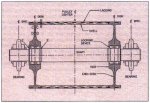
Fig. 1: Cross-section of pulley
assembly
The classical mechanics approach developed by LANGE and SCHMOLTZI is an approximate analytical approach, providing a closed-form solution for stresses in a pulley. The advantages of this method are that it is easy to program and takes a very short execution time to obtain a solution, The disadvantage is that the stress solution is not accurate at the locations near the connection region between the shell and end disks because of its poor approximation in treating the elastic coupling between these components. Specifically, the displacement of the end disk and shell are not coupled at their connection. This leads to
significant errors in the stress and strain field about the connectors as will be
shown.
The FEM has just the opposite advantages and disadvantages of the LANGE classical method. The major advantage of FEM is its ease of treating complex geometry and boundary conditions. The major disadvantage is its long execution time coupled with its need for an experienced user to generate a proper finite element mesh.
In this paper, a new method called the Modified Transfer Matrix (MTM) method is presented, This method circumvents the disadvantages of both the LANGE classical method and the conventional FEM. The MTM method proves to be a very effective and efficient approach in providing an accurate pulley assembly stress solution for any loading condition pulley.
Historically, the transfer matrix method was developed several decades ago [6] and was very popular in solving one dimensional static and dynamic problems before the advent of the FEM. Even today, this method is still useful in providing dosed form solutions to certain elasticity problems with simple boundary conditions
[7]. Although there is a limitation in handling complicated boundary conditions, such as the boundary conditions for a pulley, the solution obtained by using the transfer matrix method is exact. In this paper, it is shown that the limitation of the transfer matrix method can be overcome if the transfer matrix is reformulated by using finite element
concepts. The reformulated transfer matrix is essentially a special finite element, The new method using these special finite elements, called transfer matrix based
(TMB) finite elements, is capable of solving a class of structural elasticity problems (including the elasticity problem of a pulley), whose governing differential equations can be reduced to a set of ordinary differential
equations (ODEs). Regardless of how few of these TMB finite elements are used in a model, the solution obtained by this MTM method is generally very accurate due to the nature of the transfer matrix
method.
Based on the MTM method, a computer program for pulley stress analysis named PSTRESS 3,0 has been developed, This program can provide stress solutions and perform fatigue analysis for most pulleys, with the characteristic geometry shown in Fig. 1, The pulley can be subjected to any type of non-uniform surface pressure, sheer loading, and prescribed locking pressure.
In section 2, the general ideas for deriving TMB elements for beam (i.e. shaft), end-disk plate with variable thickness, and cylindrical shell are presented. In section 3, the assembly of these elements to model a pulley in PSTRESS
3.0 is discussed. In section 4, an example of a belt conveyor pulley is numerically solved by PSTRESS 3.0 and the results are compared with those obtained using a finely meshed FEM (ANSYS) solution.
2. TMB Finite Elements for Beam,
Disk Plate and Cylindrical Shell
Stresses and displacements in a pulley can be expressed in terms of FOURIER series with respect to the circumferential angle because of the pulley's axisymmetric geometry. Each
FOURIER component of the solutions can be determined by solving a set of corresponding governing differential equations, which are uncoupled with the governing equations for other Fourier components. In Appendices A, B
and C, it is shown that the governing equations for Fourier components for shaft, end-disk plate with non-uniform thickness, arid cylindrical shell of a pulley can be reduced to a set of ODEs of the first order respectively. The general solutions to these ODEs can be expressed in terms of the transfer matrix. By following the procedure described in Appendix D, the general solutions can be reorganized in a finite element form as below
KmDm = Fint m + Fext m (1)
where Km is the TMB element stiffness matrix, Dm is the element displacement vector, Fint m
is the element internal force vector, Fext m is the element external force vector, and the subscript
"m" denotes the FOURIER component number, The detailed procedures of developing TMB elements for shaft, end-disk and cylindrical shell are given in Appendices A, B and C, respectively.
Remarks;
As seen in the above discussion, the general solution to the governing differential equations for a pulley can be finally transformed into a finite-element form. This allows us to exploit many finite element analysis (FEA) capabilities to resolve pulley stresses using our MTM method, The most valuable
FEA capability to be employed is the way of treating complicated boundary conditions. Therefore, using the MINI method, we can easily take into account the elastic coupling between the rim and the end-disk by following
FEA assembly procedures, and implement the locking assembly pressure by using the
FEA approach of treating mechanical Interference between two bodies. Both of these problems cannot be easily or precisely handled by most classical
methods.
3. Assembly of TMB Elements for a
Pulley Model in PSTRESS 3.0
In PSTRESS 3.0, the above derived TMB beam, disk plate and cylindrical shell element stiffness matrices are brought together to font a global stiffness matrix for a pulley in essentially the same way as that in conventional FEM, However, care must be taken at two locations, where special element assembly methods are required.
The first location is the connection region between the shell and the disk shown in Fig, 2a, where the finite dimension of the joint has to be taken into account in the stiffness matrix. The conventional way of treating the whole region as a single node would cause significant error in stress solutions near this region. One of the reasonable ways of
providing correct elastic stiffness to connect the rim and the disk is treating the whole region as a special element by applying a substructure method. In
PSTRESS 3.0, such a special element shown in Fig. 2b is developed.
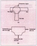
Fig. 2: Connecting element
between rim and end-disk
The second location is the connection point between the locking device and the shaft, One thing that must be kept in mind
when assembling elements in this location is that the final solution consists of many
FOURIER components, of which the shaft element only contributes to the FOURIER components of m = 0,1 and -1. In fact, in a pulley structure, the shaft deformation is governed only by these three
FOURIER components due to its slender geometry. For the component of m = 0, the corresponding shaft deformation can be exactly modeled by a
TMB cylindrical shell element presented in Appendix C. When a TMB beam element described in Appendix A is used, representing the shaft deformation of components of
m = -1 and 1 (i.e., bending deformation), the following constraints on the deformation of the connecting point must be imposed:
| Wm = -m Vm |
(2) |
|
Um = rshaftθm |
(3) |
|
Ws = Wm |
(4) |
|
θs = θm |
(5) |
Ws and
θs are the shaft deflection and rotational angle respectively at
the connecting point, where the subscript s denotes shaft deformation. The general definitions of
Ws and
θs are given in Appendix A.
Um, Vm, Wm and
θm are disk plate displacements and rotational angle at the connecting point, where the subscript m denotes the
FOURIER component number: m = -1 or 1. The general definitions of Um,
Vm, Wm and
θm, are given in Appendix B.
rshaft is the shaft radius at The connection point.
Such constraints are easy to implement in a finite element model by using FEA static condensation or penalty methods [10]. In PSTRESS 3.0, the static condensation method is employed. Finally, it must be pointed out that the TMB beam element stiffness matrix and corresponding nodal forces must be multiplied by a factor of 2 before they are assembled into global equations, due to the difference between actual forces and harmonic forces.
4. Numerical Example
Consider the belt conveyor pulley shown in Fig, 1, which is supported on two bearings and subjected to a locking pressure of 115.71 mPa (16,778 psi) at the interface between the locking device and disk hub. The shell circumferential surface pressure and shear loading between circumferential angles of
83 and 254% are developed from unequal belt tensions T1
= 1,017.8 kN (228,800 lb) and T2
= 632.98 kN (142.300 lb) shown in Fig. 3.
The material properties and geometrical parameters of the pulley are given in Table 1, This pulley is
analyzed by using
PSTRESS 3.0, ANSYS 4.4 and CDIs derivation of LANGES classical method, respectively. Because of symmetry, only one quarter of pulley cross section is modeled.
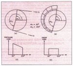
Fig. 3: Load on pulley due to
belt tension
In the PSTRESS model, the rim is modeled with 2 TMB elements, the disk is modeled
with 6
TMB elements, the shaft is modeled with 3 TMB elements, and 71 FOURIER components are used. The reason for using more TMB elements for the disk is the necessity of taking account of the non-uniform thickness of the disk. In the ANSYS
FEA model, 5,000 axisymmetric structural solid elements (with non axis-symmetric loading) are employed in the 2-0 cross-section. The use of the ANSYS FEM package to analyze a pulley is discussed in [5].
| Material Property |
|
| Young's modulus, MPSI |
30 |
| Poisson's ratio |
0.3 |
| Rim Geometry |
|
| Rim length, inches |
82 |
| Rim outer diameter, inches |
54 |
| Rim thickness, inches |
1.5 |
| Belt width, inches |
72 |
| Disk Geometry |
|
| Locking device width, inches |
3.3 |
| Hub outer diameter, inches |
27.6 |
| Hub inner diameter, inches |
20.27 |
| Hub width, inches |
6.7 |
| Fillet radius at hub, inches |
3.67 |
| Filet radius at rim, inches |
1.20 |
| Disk thickness between hub and rim,
inches |
|
| |
Radius |
Thickness |
| 1. |
15.610 |
1.740 |
| 2. |
16.268 |
1.487 |
| 3. |
19.321 |
1.409 |
| 4. |
22.400 |
1.217 |
| 5. |
22.742 |
1.199 |
|
|
| Shaft Geometry |
|
| Diameter, inches |
16.535 |
| Shaft length, inches |
121 |
| Distance between bearing centers, inches |
104 |
| Distance between disk centers, inches |
74.13 |
Table 1: Material properties
and geometrical parameters.
Figs. 4-7 show the PSTRESS numerical results compared with the ANSYS results. From these figures, it is seen that at location A of the rim and location
D of the disk the agreement between the results Of the MTM method and the results of the conventional FEM is good. At location B of the rim and location C of the disk the agreement is still good, but some inaccuracy is
observed, The reason may be that locations B and C are within the connection region between the rim and disk, where the 3-D stress state is more significant and cannot be fully taken into account in
2-D shell and plate theories. According to St. VENANTS principle and our experience, This
3-D stress state has only a very localized effect on pulley stress solution when the
thicknesses of rim and disk are relatively small compared with the length and radius of the rim. It must be noted that the MTM method is much more efficient
than the conventional FEM. PSTRESS 3.0 takes approximately 30 seconds to obtain a solution on an IBM PC 486, including the fatigue analysis. The FEM (ANSYS) solution takes 12-24 hours on an IBM RISC 6000 workstation.
|
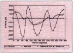
Fig. 4: Stresses at Location A
(inside of rim) PSTRESS 3.0 Analysis
|
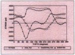
Fig. 5: Stresses at Location B
(inside of rim) PSTRESS 3.0 Analysis
|
|
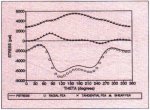
Fig. 6: Stresses at Location C
(inside of disk) PSTRESS 3.0 Analysis
|
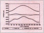
Fig. 7: Stresses at Location D
(inside of disk) PSTRESS 3.0 Analysis
|
Figs. 8-11 show the comparison of numerical results between LANGES solution and the FEM solution. Except at location A, LANGE's solution does not agree with
the FEM solution. The poor agreement is due to the errors in treating the elastic coupling between the rim and the end-disk in
LANGEs method.
|
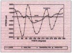
Fig. 8: Stresses at Location A
(Inside of rim) LANGE Analysis
|
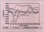
Fig. 9: Stresses at Location B
(Inside of rim) LANGE Analysis
|
|
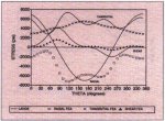
Fig. 10: Stresses at Location C
(Inside of disk) LANGE Analysis
|
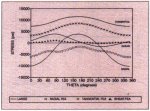
Fig. 11: Stresses at Location D
(Inside of disk) LANGE Analysis
|
Figs. 12 and 13 show both the PSTRESS and ANSYS results at two corners of the interface between the locking device and the shaft (locations E-E of Fig. 1).At these two locations,
3-D stress state is much more significant than at locations B and C. In order to produce more accurate stress solutions at the two corners, we introduce stress concentration factors in zero and first order
FOURIER component solutions by using our empirical formulae built in PSTRESS
3.0. As seen in Figs. 12 and 13, these corrected solutions agree well with ANSYS solutions.
|
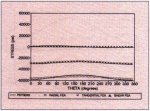
Fig. 12: Stresses at Location E
(inside of pulley) PSTRESS 3.0 Analysis
|
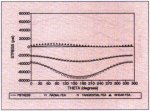
Fig. 13: Stresses at Location E (outside of pulley) PSTRESS 3.0 Analysis
|
5. Conclusions
A new pulley stress analysis method which is based on reformulated transfer matrix has been developed. An accurate solution
can be obtained by using this method. Three transfer-matrix-based elements for the shaft, disk plate and cylindrical shell
have been developed. A numerical example has been given, which demonstrates the merits of this new method.
References
- LANGE, H.: Investigations on Stress in Belt Conveyor Pul leys; Doctoral thesis, Technical University Hannover, 1963.
- SCHMOLTZI, W.: The Design
of Conveyor Belt Pulleys with Continuous Shafts; Doctoral thesis, Technical
University, Hannover 1974.
- V0DSTRCIL, P.: Analysis of Belt Conveyor Pulley Using Finite Element Method; Proc. 4th
i nt. Conf. in Australia on Finite Element Methods, University of Melbourne, Aug. 18-20, 1982.
- DANIEL, W.J.T.: Development of a Conveyor Pulley Stress Analysis Package; Proc. nt. Conf. on Bulk Material Storage, Handling and Transportation, Newcastle, Aug. 22-24, 1983.
- SETHI, V. and NORDELL, L.K.: Modern Pulley Design Techniques and Failure Analysis Methods; Proceedings of SME Annual Meeting & Exhibit, Peno Nevada, USA, Feb.
15-18,1993.
- PESTEL, S.C. and LECKIE, F.A.: Matrix Methods in Elastomechanics; New York McGraw-Hill Book Co., 1963.
- YEH KAIYUAN: General Solution on Certain Problems of Elasticity with Non-Homogeneity and Variable Thickness, The Advances of Applied Mathematics and Mechanics, Vol. 1; China Academic Publishers, pp 240-273, 1987.
- BOYCE, W.E. and DIPRIMA, R.C.:
Elementary Differential Equations; Fifth Edition, John Wiley & Sons Inc., New York, 1992.
- TIMOSHENKO, S. and
WOINOWSKY-KRIEGER. S.: Theory of Plates and Shells; McGraw-Hill Book Co., Second Edition, 1959.
- COOK, R.D., MALKUS, D.S. and PLE5HA,
M.E.: Concepts and Applications of Finite Element Analysis; Third Edition, John
Wiley & Sons Inc., 1969.
Appendix A
TMB Finite Element for Beam
Fig. A1 shows forces that act on a differential beam. Loads P, M, and q are shown in their positive sense.
z is the axial coordinate.
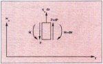
Fig. A1: Forces that act on a
differential element of beam
The equilibrium equations are
dP/dz =
-q
(A1)
dM/dz =
P
(A2)
By using TIM0SHENKOs beam theory, we have
dWs/dz = -θs +
P/kaG (A3)
dθs/dz = M/EI
(A4)
where the subscript s denotes the shaft deformation, Ws is the shaft neutral axis
displacement, -θs is the slope due to bending, dWs/dz
is the slope of the center line of the beam, k is a shape factor equal to 0.75 for circular cross section,
EI is the bending stiffness, a is the cross-section area, and G is the shear modulus.
Eqs. (A1)-(A4) can be written in a matrix form
dβ/dz = Aβ + B
(A5)
where
β = (Ws, θs, P, M)T
(A6)
B = (0, 0, -q, 0)T (A7)
and
| A = |
[
|
0 |
-1 |
1/kaG |
0 |
] |
(A8) |
| 0 |
0 |
0 |
1/EI |
| 0 |
0 |
0 |
0 |
| 0 |
0 |
1 |
0 |
where β is called state variable vector.
According to the ODE theory [8], the general solution to Eq. (A5) can be expressed as
| β(z) = T(z)β(z0)
+ T(z)
|
z
∫
z0
|
T(s)-1B(s)ds
(A9)
|
where z0 ≤ z
≤ zL, z0 and zL
are the coordinates corresponding
to two ends of the beam, and T(z) is the transfer matrix satisfying
dT/dz = AT and T(z0)
=
l
(A10)
where l is the identity matrix. Following the general procedure described in
[8]. we can obtain the following closed-form transfer matrix
| T(z) = |
[ |
1 |
z-z0 |
z-z0 |
+ |
(z-z0) |
(z-z0) |
] |
(A11) |
| kaG |
2EI |
2EI |
| 0 |
1 |
(z-z0) |
z-z0 |
| 2EI |
EI |
| 0 |
0 |
1 |
0 |
| 0 |
0 |
z-z0 |
1 |
where z0 ≤ z
≤ zL. Following the procedure described in Appendix D, we can obtain the following finite element equation, which is equivalent to
Eq. (A9)
KBMUBM =
FBMint + FBMext
(A12)
where
UBM = (Ws
(ZL), θs(ZL), Ws(Z0), θs(Z0))T
(A13)
FBMext is the beam element external force vector, FBMint
is the beam element internal force vector, and KBM is the beam element stiffness matrix, which can be expressed:
| KBM = |
[ |
12EI |
|
Symmetric |
|
] |
(A14) |
| L(1+α) |
| 6EI |
(4+α)EI |
|
|
| L(1+α) |
L(1+α) |
|
|
| -12EI |
-6EI |
12EI |
|
| L(1+α) |
L(1+α) |
L(1+α) |
|
| 6EI |
(2-α)EI |
-6EI |
(a+α)EI |
| L(1+α) |
L(1+α) |
L(1+α) |
L(1+α) |
Where
α = 12EI/LkaG
and L = ZL - Z0
(A15)
Remarks:
It is not surprising to note that the TMB finite element stiffness matrix for a beam derived as Eq. (A14) is identical to the beam stiffness matrix derived by using conventional finite element method because the polynomial-type trial function used in conventional FEM exactly represents the actual beam displacement. However, for other types of structures such as plate and shell, the TMB element stiffness matrices may not be the same as the conventional finite element stiffness matrices.
Appendix B
TMB Finite Element for Disk Plate with Variable Thickness
B.1 TMB Bending Element
Fig. B1 shows a differential element of plate subjected to bending loads. x, y and z are Cartesian coordinates with z coinciding with pulley axial direction, x horizontal direction, and y vertical direction.
r and are disk cylindrical coordinates. Loads Qr, Q, Mr, M and Mr
are shown in their positive sense.
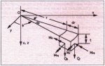
Fig. B1: Bending forces that act
on a different element of plate
The equilibrium equations are:
|
Qr = |
∂Mr
|
+ |
Mr-M |
- |
1 |
∂Mr
|
(B1) |
| ∂r |
r |
r |
∂ |
| Q
= |
∂Mr
|
+2 |
Mr
|
- |
1 |
∂M
|
(B2) |
| ∂r |
r |
r |
∂ |
| ∂Qr |
+ |
Qr
|
- |
1 |
∂Q
|
=
g(r, ) |
(B3) |
| ∂r |
r |
r |
∂ |
where g is the external transverse force acting on the neutral surface of the plate, and equations representing the force-deformation relationship are:
| Mr
= -D
|
[ |
∂u |
+ |
( |
1 |
∂u |
+ |
1 |
∂u |
)] |
(B4) |
| ∂r |
r |
∂r |
r |
∂ |
|
M = -D
|
[ |
|
∂u |
+ |
1 |
∂u |
+ |
1 |
∂u |
] |
(B5) |
| ∂r |
r |
∂r |
r |
∂ |
|
Mr
= D(1-)
|
[ |
1 |
∂u |
- |
1 |
∂u |
] |
(B6) |
| r |
∂r∂ |
r |
∂ |
where U is the plate neutral surface transverse displacement (see Fig.
B1), is the POISSON's ratio,
D = Et/12(1 - )
(B7)
E is the YOUNG's modulus, t is the thickness of the plate, which is a function of r, Within the element, we
assume
t = crp
(B8)
where a and p are constants.
Also, we assume the following FOURIER series for the components of displacement and forces
| u = |
∞
Σ
m=0 |
umcosm + |
∞
Σ
m=1 |
u-msinm
(B9) |
| g = |
∞
Σ
m=0 |
gmcosm + |
∞
Σ
m=1 |
g-msinm (B10) |
| Qr = |
∞
Σ
m=0 |
Qrmcosm + |
∞
Σ
m=1 |
Qr,-msinm (B11) |
| Q = |
∞
Σ
m=1 |
Qmsinm + |
∞
Σ
m=0 |
Q,-mcosm (B12) |
| Mr = |
∞
Σ
m=0 |
Mrmcosm + |
∞
Σ
m=1 |
Mr,-msinm (B13) |
| M = |
∞
Σ
m=0 |
Mmcosm + |
∞
Σ
m=1 |
M,-msinm (B14) |
| Mr = |
∞
Σ
m=1 |
Mrsinm + |
∞
Σ
m=0 |
Mr,-mcosm (B15) |
where um, Pm,
Qrm, Qm, Mrm, Mm, Mrm (m=O.1,2,...)
are functions of r only. Substituting Eqs. (89)-(B15) into Eqs. (B1)-(B6), we have the following ordinary differential equations
| Qrm = M'rm + |
1 |
(Mrm - Mm) - |
m |
Mrm |
(B16) |
| r |
r |
| Qm
= M'rm + |
2 |
Mrm
+ |
m |
Mm |
(B17) |
| r |
r |
|
Q'rm + |
1 |
Qrm
- |
m |
Qm
= gm |
(B18) |
| r |
r |
| Mrm = -D |
[ |
u"m + |
( |
1 |
u'm - |
m |
um |
)] |
(B19) |
| r |
r |
| Mm
= - D
|
[ |
u"m + |
1 |
u'm - |
m |
um |
] |
(B20) |
| r |
r |
|
Mrm =
D(1-) |
[ |
- |
m |
u'm
+ |
m |
um |
] |
(B21) |
| r |
r |
where m = 0, 1, 2, ..., and the prime represents derivative with respect to r. Introducing the following state variables
γm = (um, θm,
rm, Mrm)T (B22)
Where
| θm = u'm
|
(B23) |
| mrm = -2πr
Mrm |
(B24) |
| Vrm = 2πr (Qm - m/r Mrm) |
(B25) |
Eliminating five variables,
Mrm, Mm, Mrm, Qrm and Qm
among Eqs. (B16)-(B21) and (B23)-(B25), we can obtain the following matrix-form equation
dγm/dr = Am
γm + Bm (m = 0, 1, 2, ...) (B26)
Where Am =
| [ |
0 |
1 |
0 |
0 |
] |
(B27) |
| m |
_ |
0 |
1 |
| r |
r |
2πDr |
| 2πDm(2 - 2 + m
- m) |
-2πDm(3 - 2 -
) |
_ 1 |
m |
| r |
r |
r |
r |
| 2πDm(-3 + 2 +
) |
2πD(1 - + 2m -
2m) |
-1 |
(1 - ) |
| r |
r |
r |
Bm = (0, 0, 2πrgm, 0)T
(B28)
Therefore, following the procedure described in Appendix D, we can obtain the following
finite element equation for a circular plate ring (r0 ≤ r ≤
rL) with variable thickness and subjected to harmonic bending load
KBD mUBDm
= FBDint m + FBDext m
(B29)
Where
UBDm = (ULm,
Lm, Uom, θ0m)T
(B30)
KBD m is the plate element bending stiffness matrix, FBDext m
is the element external force vector, FBDint m is the element internal force
vector, the subscript L and 0 denote locations at r = rL and r0,
respectively, and m denotes the FOURIER component number. Due to the complexity in
deriving the transfer matrix for Eq. (B26), it is much more difficult to obtain a closed-form expression
for KBD m of Eq. (B29) than for KBM of Eq. (A12). Instead, we can very accurately calculate
KBD m by using our computer program of PSTRESS 3.0 mentioned in Remark ii of Appendix D.
B.2 TBM Plane Stress Element
Fig. B2 shows a differential element of plate subjected to in-plane loading. Loads
Nr, N, and Nr are shown in their positive sense.
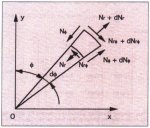
Fig. B2: In-plane forces that
act on a differential element of plate
The definitions of x, y, Z,
r and are the same as in section B.1. The equilibrium equations are
| ∂Nr |
+ |
Nr - N |
+ |
1 |
∂Nr |
= 0 (B31) |
| ∂r |
r |
r |
∂ |
| ∂Nr |
+ 2 |
Nr |
+ |
1 |
∂N |
= 0 (B32) |
| ∂r |
r |
r |
∂ |
The equations for force-deformation relationship are
| Nr = |
Et |
( |
∂w |
+ |
1 |
∂v |
+ |
w |
) |
(B33) |
| (1 - ) |
∂r |
r |
∂ |
r |
| N = |
Et |
( |
|
∂w |
+ |
1 |
∂v |
+ |
w |
) |
(B34) |
| (1 - ) |
∂r |
r |
∂ |
r |
| Nr = |
Et |
( |
∂v |
+ |
1 |
∂w |
- |
v |
) |
(B35) |
| 2(1 + ) |
∂r |
r |
∂θ |
r |
where the definitions of , E and t are the same as in section B.1, arid v and w are the displacements of the neutral surface in circumferential and radial directions, respectively.
We assume the following FOURIER series for the components of displacements and forces
| v = |
∞
Σ
m=1 |
vmsinm + |
∞
Σ
m=0 |
v-mcosm (B36) |
| w = |
∞
Σ
m=0 |
wmcosm + |
∞
Σ
m=1 |
w-msinm (B37) |
| Nr = |
∞
Σ
m=0 |
Nrmcosm + |
∞
Σ
m=1 |
Nr,-msinm (B38) |
| N = |
∞
Σ
m=0 |
Nmcosm + |
∞
Σ
m=1 |
N,-msinm (B39) |
| Nr = |
∞
Σ
m=1 |
Nrmsinm + |
∞
Σ
m=0 |
Nrmcosm (B40) |
where vmwm, Nrm, Nm and Nrm(m
= 0,1,2, ...) are functions of r only. Substituting Eqs. (B36)-(B40) into Eqs.
(B31)-(B35), we have the following ordinary differential equations
|
N'rm + |
1 |
(Nrm
- Nrm)+ |
m |
Nrm
= 0 |
(B41) |
| r |
r |
| N'rm
+ |
2 |
Nrm - |
m |
Nm
= 0 |
(B42) |
| r |
r |
| Nrm = |
Et |
[ |
w'm
+ |
( |
m |
vm
+ |
1 |
wm |
)] |
(B43) |
| (1 - ) |
r |
r |
| Nm
= |
Et |
[ |
w'm
+ |
m |
vm
+ |
1 |
wm |
] |
(B44) |
| (1 - ) |
r |
r |
| Nrm
= |
Et |
[ |
v'm
- |
m |
wm
- |
1 |
vm |
] |
(B45) |
| 2(1 + ) |
r |
r |
where m = 0, 1, 2, 3,.... Introducing the following state variables
ηm = (wm, vm, 2πrNrm
, 2πrNrm)T
(B46)
and eliminating Nm among Eqs. (B41)-(B45). we obtain
dηm/dr = Cm
ηm (m = 0, 1, 2, ...)
(B47)
where
| Cm
= |
[ |
_ |
_ m |
1- |
0 |
] |
(B48) |
| r |
r |
2πEtr |
| m |
1 |
0 |
1 + |
| r |
r |
2πEtr |
| 2πEt |
2πEtm |
_ 1 - |
_ m |
| r |
r |
r |
r |
| 2πEtm |
2πEtm |
m |
_ 2 |
| r |
r |
r |
r |
Thus, following the similar procedure in deriving Eq.
(B29) , we can finally derive the following TMB finite element equation for a circular ring
(r0 ≤ r ≤ rL) with variable thickness, subjected to in-plane harmonic loading
KPN m UPNm
= FPNint m + FPNext m
(B49)
where
UPNm = (WLm,
VLm, W0m, V0m)T
(B50)
KPN m is the element plane-stress stiffness matrix, FPNext m
is the element external force vector, FPNint m is the element internal force vector, and the subscript L and C denote locations at
r =
rL and r0 respectively, and m denotes the FOURIER component number.
Combining Eq. (B29) and Eq. (B49), we can form a TMB shell element for disk plate, which is subjected to both bending and
in-plane loading
KDK m UDKm =
FDkint m + FDKext m
(B51)
where KDK m is the disk element stiffness matrix, UDKm
is the element displacement vector, FDKext m is the element extemal force vector, and
FDkint m is the element internal force vector. They can be calculated by the following formulae
| UDKm = (ULm, VLm,
WLm, θLm, U0m, V0m,
W0m, θ0m)T
|
(B52)
|
| KDK m = ST1KBD mS1
+ ST2KPN mS2
|
(B53)
|
| FDKint m =
ST1FBDint m + ST2FPNint m
|
(B54)
|
| FDKext m =
ST1 FBDext m + ST2 FPNext m
|
(B55)
|
| S1 = |
[ |
1 |
0 |
0 |
0 |
0 |
0 |
0 |
0 |
] |
(B56) |
| 0 |
0 |
0 |
1 |
0 |
0 |
0 |
0 |
| 0 |
0 |
0 |
0 |
1 |
0 |
0 |
0 |
| 0 |
0 |
0 |
0 |
0 |
0 |
0 |
1 |
Remarks:
- Any other state variables than
those defined in Eq. (B22) and Eq. (B46) cannot be employed because they may lead to
incorrect element stiffness matrices and force vectors due to the violation of
MAXWELL'S reciprocal theorem.
- Stiffness matrices obtained from
transfer matrices must be symmetric. Any mistakes in choosing state variables, in
deriving equations, and/or in numerical programming may lead to asymmetric stiffness
matrices.
- If the stress calculation is
desired, we can follow the following steps
- calculate values of state
variables at element nodes,
- use transfer matrix and Eq.
(D3) to calculate values of state variables at any interior location of the
element, where stress values are desired,
- calculate first derivatives
of state variables at desired locations by using Eq. (B26) and Eq. (B47),
- calculate Mrm,
Mm, Mrm, Nrm, Nm and Nrm
by using Eqs. (B19)-(B21) and Eqs. (B43)-(B45), and
- calculate FOURIER components
of stresses by using calculated forces in step d.
Appendix C
TMB Finite Element for Cylindrical Shell
Fig. C1 shows forces acting on a differential element of a cylindrical shell with constant thickness
t and radius R, z and are cylindrical coordinates. Loads N1, N2,
S, Q1, Q2, M1, M2 and M12 are shown in their positive sense.
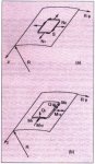
Fig. C1: Forces that act on a
differential element of cylindrical
The equilibrium equations, according to
[9] are
| |
|
∂N1 |
+ |
∂S |
+ fz =
0 |
(C1) |
| |
|
∂z |
R∂ |
| |
|
∂N2 |
+ |
∂S |
+ f =
0 |
(C2) |
| |
|
R∂ |
∂z |
| _ N2 |
+ |
∂Q1 |
+ |
∂Q2 |
+ fr =
0 |
(C3) |
| R |
∂z |
R∂ |
| Q2
= |
∂M12 |
+ |
∂M2 |
|
(C4) |
| ∂z |
R∂ |
| Q1
= |
∂M1 |
+ |
∂M12 |
|
(C5) |
| ∂z |
R∂ |
where fz, f
and fr are external loads acting on the neutral surface of the shell in axial,
circumferential and radial directions respectively, and the equations for force-displacement relationship, according to
[9]. are
| N1 = |
Et |
|
( |
∂u |
+ |
∂v |
+ |
w |
) |
(C6) |
| (1-) |
∂z |
R∂ |
R |
| N2 = |
Et |
( |
|
∂u |
+ |
∂v |
+ |
w |
) |
(C7) |
| (1-) |
∂z |
R∂ |
R |
| |
|
S
= |
Et |
( |
∂u |
+ |
∂v |
) |
(C8) |
| |
(1-2) |
R∂ |
∂z |
| |
|
M1
= -D |
( |
∂w |
+ |
∂u |
) |
(C9) |
| |
|
∂z |
R∂ |
| |
|
M2
= -D |
( |
|
∂w |
+ |
∂u |
) |
(C10) |
| |
∂z |
R∂ |
| |
|
|
|
M12 = -(1 - )D |
∂w |
|
(C11) |
| |
|
|
|
R∂z∂ |
|
where u, v and w are shell neutral surface displacements in axial, circumferential and radial directions, respectively,
D = Et/12(1 - )
the definitions of E and are the same as in section B, and t is
the constant shell thickness. We assume the following FOURIER
components of displacements and forces
| fz = |
∞
Σ
m=0 |
fzmcosm + |
∞
Σ
m=1 |
fz,-msinm |
(C12) |
| f = |
∞
Σ
m=1 |
fmsinm + |
∞
Σ
m=0 |
f,-mcosm |
(C13) |
| fr = |
∞
Σ
m=0 |
frmcosm + |
∞
Σ
m=1 |
fr,-msinm |
(C14) |
| u = |
∞
Σ
m=0 |
umcosm + |
∞
Σ
m=1 |
u-msinm |
(C15) |
| v = |
∞
Σ
m=1 |
vmsinm + |
∞
Σ
m=0 |
v-mcosm |
(C16) |
| w = |
∞
Σ
m=0 |
wmcosm + |
∞
Σ
m=1 |
w-msinm |
(C17) |
| N1 = |
∞
Σ
m=0 |
N1mcosm + |
∞
Σ
m=1 |
N1,-msinm |
(C18) |
| N2 = |
∞
Σ
m=0 |
N2mcosm + |
∞
Σ
m=1 |
N2,-msinm |
(C19) |
| S = |
∞
Σ
m=1 |
Smsinm + |
∞
Σ
m=0 |
S-mcosm |
(C20) |
| M1 = |
∞
Σ
m=0 |
M1mcosm + |
∞
Σ
m=1 |
M1,-msinm |
(C21) |
| M2 = |
∞
Σ
m=0 |
M2mcosm + |
∞
Σ
m=1 |
M2,-msinm |
(C22) |
| M12 = |
∞
Σ
m=1 |
M12msinm + |
∞
Σ
m=0 |
M12,-mcosm |
(C23) |
| Q1 = |
∞
Σ
m=0 |
Q1mcosm + |
∞
Σ
m=1 |
Q1,-msinm |
(C24) |
| Q2 = |
∞
Σ
m=1 |
Q2msinm + |
∞
Σ
m=0 |
Q2,-mcosm |
(C25) |
where all FOURIER coefficients are functions of z only. Substituting Eqs.
(C12)-(C25) into Eqs. (C1)-(C11), introducing the following state variables
ξm = (Um, Vm, Wm,
θm, 2πRN1m, 2πRSm,
2πRV1m, 2πRM1m)T
(C26)
Where
θm = -W'm
(C27)
and
V1m = Q1m
+ m/R M12m (C28)
and eliminating five variables,
N2m, M2m, M12m, Q1m and Q2m we can finally obtain the following matrix-form equation after a
long tedious procedure of mathematical derivation
dξm/dz = Jmξm
+ Im (m = 0, 1, 2, ...) (C29)
Where
| Jm
=
|
[ |
0 |
_ m |
_ |
0 |
1 - |
0 |
0 |
0 |
] |
(C30) |
| R |
R |
2πEtR |
| m |
0 |
0 |
0 |
0 |
1 + |
0 |
0 |
| R |
πEtR |
| 0 |
0 |
0 |
-1 |
0 |
0 |
0 |
0 |
| 0 |
0 |
_ m |
0 |
0 |
0 |
0 |
6(1 - ) |
| R |
πEtR |
| 0 |
0 |
0 |
0 |
0 |
_ m |
0 |
0 |
| R |
| 0 |
πEtm |
2πEtm |
0 |
m |
0 |
0 |
0 |
| R |
R |
R |
| 0 |
2πEtm |
2πEt |
( |
1 + |
tm4 |
) |
0 |
|
0 |
0 |
m |
| R |
R |
12R |
R |
R |
| 0 |
0 |
0 |
πEtR |
0 |
0 |
1 |
0 |
| 3(1+)R |
and
Im = (0, 0, 0, 0, -
2πRfzm, -2πRfm, 2πRfrm, 0)T
(C31)
Therefore, according to the conclusions of
Appendix D, the transfer matrix for Eq. (C29) can be obtained by the computer program developed in PSTRESS 3.0, Based on the transfer matrix, the TMB finite element for cylindrical shell with
z0 ≤ z ≤ zL can be derived by following the procedure described in Appendix
D, and the result can be expressed by
KCS m UCSm
= FCSint m + FCSext m
(C32)
where
UCSm = (ULm,
VLm, WLm, θLm, U0m, V0m,
W0m, θ0m)T
(C33)
KCS m is the cylindrical-shell stiffness matrix,
FCSext m is the element external force vector, FCSint
m is the element internal force vector, and the subscripts L and 0 denote locations at z - zL, and z = z0, respectively, and m denotes the
FOURIER component number.
If stress calculation for cylindrical shell is desired, we can follow the similar procedure described in
Remark vi of section B.
Appendix D
Procedure of Deriving TMB Finite Element
In Appendices A, B and C, it is shown that the governing equations for FOURIER components for shaft, end-disk plate with nonuniform thickness, and cylindrical shell of a pulley can be reduced to a set of ODEs of first order respectively, and these ODEs can be finally unified as the following form
dψm/ds =
Hm(s)ψm + Lm
(m = 0, 1, 2, ...) (D1)
where the subscript m denotes the
ordinary number of FOURIER components, Hm is a 2n x2n matrix. Lm
is a 2n x 1 vector containing external loads, ψm is the state variable
vector defined as
ψm = (UTm,
FTm)T (D2)
Um is an n x 1 vector containing generalized displacements,
Fm an n x 1 vector containing corresponding generalized internal forces, and s
is an axial or radial coordinate of the pulley, which is assumed within the range of
s0 ≤ s ≤ sL, where
s0
and sL are corresponding to two ends of a pulley component section (i,e, element).
Because Eq. (D1) is linear, the general solution is obtainable. By using the theory of
ODE [8], the general solution to Eq. (D1) can be written as
| ψm(S) = Tm(S)
ψm(s0) + Tm(S) |
s
∫
s0 |
Tm(X)-1Lm
(x)dx
(D3) |
where Tm(s)
is a 2n x 2n matrix called transfer matrix satisfying
dTm/ds = HmTm
and Tm(s0) = I (D4)
where I is the identity matrix, For any set of linear ordinary differential equations, which can be expressed in the form of Eq.
(D1), there exists a unique 2n x 2n transfer matrix Tm(s)
satisfying Eq. (D4). If Eq. (D1) is a set of constant ODEs (i.e., Hm is independent of s) or it can be transformed into a set of constant ODEs, a closed-form transfer matrix
Tm(s) is obtainable. The general procedure of deriving Tm(s)
is discussed in many textbooks, such as the one by BOYCE and DIPRIMA [8]. In what follows in this section, it is shown that a special finite element (i.e., TMB element) can be developed from Eq. (D3).
Let us consider a section of pulley, which is located in
s0 ≤ s ≤ sL, and let
| Tm(SL)= |
[ |
TUU |
TUF |
] |
(D5) |
| TFU |
TFF |
| ψm(SL)= |
[ |
UL |
] |
(D6) |
| Fint L |
| ψm(S0)= |
[ |
Uo |
] |
(D7) |
| -Fint 0 |
|
Pm = Tm(sL)
|
sL
∫
s0
|
Tm(X)-1 B(x)dx
(D8)
|
Where
| UL = Um(SL)
|
(D9) |
| Uo = Um(S0)
|
(D10) |
| Fint L = Fm(SL) |
(D11) |
| Fint 0 = -Fm(S0) |
(D12) |
Then Eq. (D3) can be rewritten as
| [ |
UL |
] |
= |
[ |
TUU |
-TUF |
][ |
Fint L |
] |
+
Pm (D13) |
| Fint L |
TFU |
-TFF |
Fint 0 |
Reorganizing Eq. (D13), we have
| [ |
I |
-TUU |
][ |
UL |
] |
= |
[ |
0 |
-TUF |
][ |
Fint L |
] |
+
Pm (D14) |
| 0 |
-TFU |
U0 |
-I |
-TFF |
Fint 0 |
from which we can obtain
KmDm = Fint m + Fext m
(D15)
Where
| Km
= |
[ |
0 |
-TUF |
]-1[ |
I |
-TUU |
] |
(D16) |
| -I |
-TFF |
o |
-TFU |
| Dm
= (UTL, UT0)T
(D17) |
| Fint
m = |
[ |
Fint L |
] |
|
(D18) |
| Fint
0 |
| Fext
m = |
[ |
0 |
-TUF |
]-1 |
Pm |
(D19) |
| -1 |
-TFF |
It is seen that Eq. (D15) is formulated in a finite-element form, where Km
is element stiffness matrix, Dm
is the element displacement vector, Fint
m is the element internal force vector, and
Fext m
is the element external force vector, The detailed procedures of developing TMB elements for shaft, end-disk and cylindrical shell are given in Appendices A, B
and C, respectively.
Remarks:
- It is noted that in developing TMB finite elements the trial function for representing element displacement field is not required. This is the feature that distinguishes the MTM method from the conventional
finite element method.
- In general, for any type of structures, whose governing differential equations can be reduced to the form of
Eq. (D1), which can be further transformed into a set of constant ODEs, the corresponding transfer matrix
Tm(s) of Eq.
(D3) can be derived following some standard procedure described in [8]. In most cases, the procedure of deriving
Tm(S) can be fulfilled by using a computer program, and
Pm defined in Eq.
(D8) can be evaluated analytically or numerically; and Therefore, a computer program can be made, where the input is the matrix
Hm and the external loads, and the output is the
TMB element stiffness matrix and element external force vector. In this program, there is no discretization error in computing TMB element stiffness matrix. As a FORTRAN subroutine, such a computer program has been
developed in PSTRESS 3.0.